Week 3 - Adiabatic Flame Temperature calculation
Equivalence Ratio-Equivalence ratio is ratios of fuel by air of the mixture and stoichiometric fuel by air ratio of the mixture.
The Equivalence ratio for stoichiometric mixture is 1 (`phi=1`).
The Equivalence ratio of the lean mixture is less than 1 (`phi <1`).
The Equivalence ratio of the rich mixture is greater than 1 (`phi>1`).
Adiabatic Flame Temperature- The temperature attained when all of the chemical reaction heat released heats combustion products.
1) Adiabatic flame temperature variation with Equivalence ratio (In constant volume-chamber) :
For combustion in constant pressure chamber, the internal energy of the product and reactant has to be equal in order to get the Adiabatic flame temperature.
`DeltaU_(Product)=DeltaU_(Reactant)`
`H_(Product)-H_(Reactant) - (n_p*T-n_r*T_(std))*R=0`
Enthalpy of the reactant and product are calculated with the help of naza polynomial, and the value of the coefficients was obtained from berkeleyedu website.
The equation of the Enthalpy is given as:
`H=(a_1*T+a_2*T^2+a_3*T^3+a_4*T^4+a_5*T^5+a_6/T)*R*T`
The Adiabatic Flame temperature is calculated numerically with the help of Newton Raphson method and with Cantera codes.
The equivalence ratio was varied from 0.5 to 1.5.
The code is attached below:
import matplotlib.pyplot as plt
import numpy as np
import math
def h(T, coeff):
R=8.314 #J/mol-K
a1=coeff[0]
a2=coeff[1]
a3=coeff[2]
a4=coeff[3]
a5=coeff[4]
a6=coeff[5]
return (a1*T + a2*(pow(T,2)/2) + a3*(pow(T,3)/3) + a4*(pow(T,4)/4) + a5*(pow(T,5)/5) + a6)*R
ch4_coeffs_l = [5.14987613E+00, -1.36709788E-02, 4.91800599E-05, -4.84743026E-08, 1.66693956E-11, -1.02466476E+04, -4.64130376E+00]
o2_coeffs_h = [3.28253784E+00, 1.48308754E-03, -7.57966669E-07, 2.09470555E-10, -2.16717794E-14, -1.08845772E+03, 5.45323129E+00]
o2_coeffs_l = [3.78245636E+00, -2.99673416E-03, 9.84730201E-06, -9.68129509E-09, 3.24372837E-12, -1.06394356E+03, 3.65767573E+00]
n2_coeffs_h = [0.02926640E+02, 0.14879768E-02, -0.05684760E-05, 0.10097038E-09, -0.06753351E-13, -0.09227977E+04, 0.05980528E+02]
n2_coeffs_l = [0.03298677E+02, 0.14082404E-02, -0.03963222E-04, 0.05641515E-07, -0.02444854E-10, -0.10208999E+04, 0.03950372E+02]
co2_coeffs_h = [3.85746029E+00, 4.41437026E-03, -2.21481404E-06, 5.23490188E-10, -4.72084164E-14, -4.87591660E+04, 2.27163806E+00]
h20_coeffs_h = [3.03399249E+00, 2.17691804E-03, -1.64072518E-07, -9.70419870E-11, 1.68200992E-14, -3.00042971E+04, 4.96677010E+00]
co_coeffs_h = [2.71518561E+00, 2.06252743E-03, -9.98825771E-07, 2.30053008E-10, -2.03647716E-14, -1.41518724E+04, 7.81868772E+00]
def f(T,phi):
R=8.314
h_co2_p=h(T,co2_coeffs_h)
h_h2o_p=h(T,h20_coeffs_h)
h_n2_p=h(T,n2_coeffs_h)
h_o2_p=h(T,o2_coeffs_h)
h_co_p=h(T,co_coeffs_h)
#Lean Mixture
if phi<1:
h_products=h_co2_p + 2*h_h2o_p + (7.52/phi)*h_n2_p + (2/phi - 2)*h_o2_p
n_p=9.52/phi + 1
#Rich Mixture
elif phi>1:
h_products=(4/phi -3)*h_co2_p + (4-4/phi)*h_co_p + 2*h_h2o_p + (7.52/phi)*h_n2_p
n_p=7.52/phi + 3
#Stoichiometric Mixture
else:
h_products=h_co2_p + 2*h_h2o_p + 7.52*h_n2_p
n_p=10.52
print(h_products)
Tstd=298.15
h_ch4_r=h(Tstd,ch4_coeffs_l)
h_o2_r=h(Tstd,o2_coeffs_l)
h_n2_r=h(Tstd,n2_coeffs_l)
h_reactants=h_ch4_r+(2/phi)*h_o2_r+(7.52/phi)*h_n2_r
n_r=1+9.52/phi
print(h_reactants)
return h_products-h_reactants - (n_p*T-n_r*Tstd)*R
def fprime(T,phi):
return (f(T+1e-06,phi)-f(T,phi))/1e-06
phi=np.linspace(0.5,1.5,num=21)
l=len(phi)
T_guess =np.ones(l)
tol=1e-06
ct=np.zeros(l)
alpha=0.5
for i in range(l):
while (abs(f(T_guess[i],phi[i]))>tol):
T_guess[i]=T_guess[i] - alpha*(f(T_guess[i],phi[i])/fprime(T_guess[i],phi[i]))
ct[i]=ct[i]+1
print(ct)
print(T_guess)
T_ct=np.ones(l)
#Cantera
import cantera as ct
for i in range(l):
gas=ct.Solution('gri30.xml')
gas.TPX=298.15,101325,{'CH4':1,'O2':2/phi[i],'N2':7.52/phi[i]}
gas.equilibrate('UV','auto')
T_ct[i]=gas.T
print(T_ct)
#Plot
plt.title('Effect of Equivalence Ratio on Adiabatic Flame Temperature of methane')
plt.plot(phi,T_guess,color='green',label="Newton Raphson")
plt.plot(phi,T_ct,color='blue',label="Cantera")
plt.grid('on')
plt.xlabel('Equivalence Ratio')
plt.ylabel('Adiabatic Flame Temperature')
plt.legend(loc='lower right', shadow=True)
plt.show()
The Figure 1 is the plot obtained after running the code.
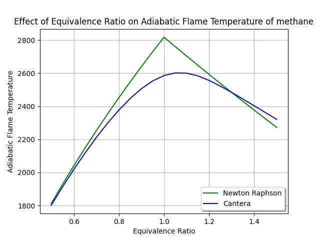
Figure 1
Both line graphs seems to follow same trend. It can be seen that the adiabatic flame temperature acheived is by using cantera is lower than that calculated numerically. This is because during actual combustion many other chemical species are created other than the ones in the balanced equations.
2) Flame temperature variation with Heat loss (In constant pressure-chamber) :
For combustion in a constant pressure chamber the difference in enthalpy of is product and reactant is equal to the heat loss.
`H_p-H_r=HeatLoss`
The maximum possible heat loss in the combustion is the lower heating value of the reaction. The relation between heat loss and Lower heating value can be given as
Heat_Loss=Heat_Loss_Factor*LHV
The Code for this probem is:
import matplotlib.pyplot as plt
import numpy as np
import math

def h(T, coeff):

	R=8.314 #J/mol-K
	a1=coeff[0]
	a2=coeff[1]
	a3=coeff[2]
	a4=coeff[3]
	a5=coeff[4]
	a6=coeff[5]

	return (a1*T + a2*(pow(T,2)/2) + a3*(pow(T,3)/3) + a4*(pow(T,4)/4) + a5*(pow(T,5)/5) + a6)*R

ch4_coeffs_l = [5.14987613E+00, -1.36709788E-02, 4.91800599E-05, -4.84743026E-08, 1.66693956E-11, -1.02466476E+04, -4.64130376E+00]
o2_coeffs_l = [3.78245636E+00, -2.99673416E-03, 9.84730201E-06, -9.68129509E-09, 3.24372837E-12, -1.06394356E+03, 3.65767573E+00 ]
n2_coeffs_h = [0.02926640E+02, 0.14879768E-02, -0.05684760E-05, 0.10097038E-09, -0.06753351E-13, -0.09227977E+04, 0.05980528E+02]
n2_coeffs_l = [0.03298677E+02, 0.14082404E-02, -0.03963222E-04, 0.05641515E-07, -0.02444854E-10, -0.10208999E+04, 0.03950372E+02]
co2_coeffs_h = [3.85746029E+00, 4.41437026E-03, -2.21481404E-06, 5.23490188E-10, -4.72084164E-14, -4.87591660E+04, 2.27163806E+00]
h20_coeffs_h = [3.03399249E+00, 2.17691804E-03, -1.64072518E-07, -9.70419870E-11, 1.68200992E-14, -3.00042971E+04, 4.96677010E+00]

def f(T,HL,LHV):
	h_co2_p=h(T,co2_coeffs_h)
	h_h2o_p=h(T,h20_coeffs_h)
	h_n2_p=h(T,n2_coeffs_h)

	h_products=h_co2_p + 2*h_h2o_p + 7.52*h_n2_p
	print(h_products)

	Tstd=298.15
	h_ch4_r=h(Tstd,ch4_coeffs_l)
	h_o2_r=h(Tstd,o2_coeffs_l)
	h_n2_r=h(Tstd,n2_coeffs_l)

	h_reactants=h_ch4_r+2*h_o2_r+7.52*h_n2_r
	print(h_reactants)

	return h_products-h_reactants+HL*LHV

def fprime(T,HL,LHV):
	return (f(T+1e-06,HL,LHV)-f(T,HL,LHV))/1e-06

T_std=298.15
LHV = h(T_std,ch4_coeffs_l) + 2*h(T_std,o2_coeffs_l) - h(T_std,co2_coeffs_h) - 2*h(T_std,h20_coeffs_h)
heat_loss=np.linspace(0,1,num=21)
l=len(heat_loss)
T_guess =np.ones(l)*1500

tol=1e-06
ct=np.zeros(l)
alpha=0.5
for i in range(l):
	while (abs(f(T_guess[i],heat_loss[i],LHV))>tol):
		T_guess[i]=T_guess[i] - alpha*(f(T_guess[i],heat_loss[i],LHV)/fprime(T_guess[i],heat_loss[i],LHV))
		ct[i]=ct[i]+1

print(ct)
print(T_guess)
plt.plot(heat_loss,T_guess,'*',color='blue')
plt.xlabel('Heat loss')
plt.ylabel('Temperature')
plt.show()
The plot obtained is as follows in figure 2:
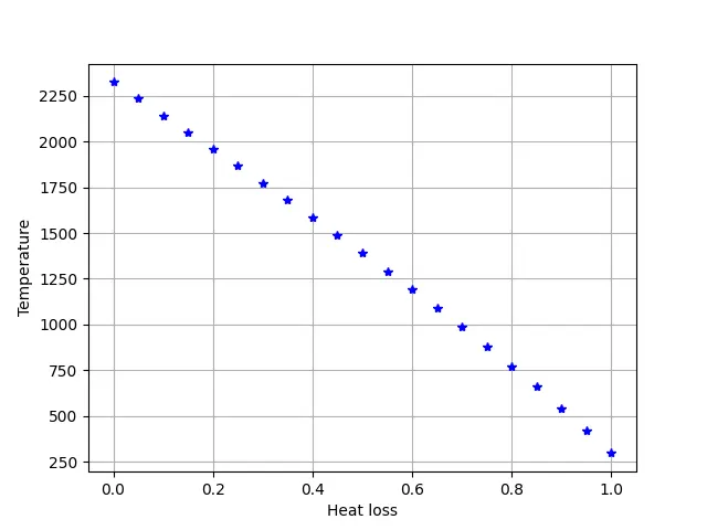
Figure 2.
It can be seen as we keep increasing the heat loss factor the Adiabatic flame temperature decreases.
3. Adiabatic flame temperature variation with respect to Alkane, Alkene, Alkyne :
The hydrocarbons used for this simulation are ethane, ethene and ethyne.
The code used to run simulation is as follows
The plot obtained can be seen in figure 3.
import matplotlib.pyplot as plt
import numpy as np
import math

def h(T, coeff):

	R=8.314 #J/mol-K
	a1=coeff[0]
	a2=coeff[1]
	a3=coeff[2]
	a4=coeff[3]
	a5=coeff[4]
	a6=coeff[5]

	return (a1*T + a2*(pow(T,2)/2) + a3*(pow(T,3)/3) + a4*(pow(T,4)/4) + a5*(pow(T,5)/5) + a6)*R

c2h6_coeffs_l = [4.29142492E+00, -5.50154270E-03, 5.99438288E-05, -7.08466285E-08, 2.68685771E-11, -1.15222055E+04, 2.66682316E+00]
c2h4_coeffs_l = [3.95920148E+00, -7.57052247E-03, 5.70990292E-05, -6.91588753E-08, 2.69884373E-11, 5.08977593E+03, 4.09733096E+00]
c2h2_coeffs_l = [8.08681094E-01, 2.33615629E-02, -3.55171815E-05, 2.80152437E-08, -8.50072974E-12, 2.64289807E+04, 1.39397051E+01]
o2_coeffs_l = [3.78245636E+00, -2.99673416E-03, 9.84730201E-06, -9.68129509E-09, 3.24372837E-12, -1.06394356E+03, 3.65767573E+00]
n2_coeffs_h = [0.02926640E+02, 0.14879768E-02, -0.05684760E-05, 0.10097038E-09, -0.06753351E-13, -0.09227977E+04, 0.05980528E+02]
n2_coeffs_l = [0.03298677E+02, 0.14082404E-02, -0.03963222E-04, 0.05641515E-07, -0.02444854E-10, -0.10208999E+04, 0.03950372E+02]
co2_coeffs_h = [3.85746029E+00, 4.41437026E-03, -2.21481404E-06, 5.23490188E-10, -4.72084164E-14, -4.87591660E+04, 2.27163806E+00]
h20_coeffs_h = [3.03399249E+00, 2.17691804E-03, -1.64072518E-07, -9.70419870E-11, 1.68200992E-14, -3.00042971E+04, 4.96677010E+00]

def f(T,n):
	#Product
	h_co2_p=h(T,co2_coeffs_h)
	h_h2o_p=h(T,h20_coeffs_h)
	h_n2_p=h(T,n2_coeffs_h)

	#Reactant
	Tstd=298.15
	h_o2_r=h(Tstd,o2_coeffs_l)
	h_n2_r=h(Tstd,n2_coeffs_l)

	h_c2h6_r=h(Tstd,c2h6_coeffs_l)
	h_c2h4_r=h(Tstd,c2h4_coeffs_l)
	h_c2h2_r=h(Tstd,c2h2_coeffs_l)

	if n==1:
		h_products=2*h_co2_p + 3*h_h2o_p + 13.16*h_n2_p
		h_reactants=h_c2h6_r+3.5*h_o2_r+13.16*h_n2_r
	elif n==2:
		h_products=2*h_co2_p + 2*h_h2o_p + 11.28*h_n2_p
		h_reactants=h_c2h4_r+3*h_o2_r+11.28*h_n2_r
	elif n==3:
		h_products=2*h_co2_p + 1*h_h2o_p + 9.4*h_n2_p
		h_reactants=h_c2h2_r+2.5*h_o2_r+9.4*h_n2_r

	return h_products-h_reactants

def fprime(T,n):
	return (f(T+1e-06,n)-f(T,n))/1e-06

n=np.linspace(1,3,num=3)
fuels=['C2H6','C2H4','C2H2']
l=len(n)
tol=1e-06
T_guess =np.ones(l)*1500
ct=np.zeros(l)
alpha=0.5

for i in range(l):
	while (abs(f(T_guess[i],n[i]))>tol):
		T_guess[i]=T_guess[i] - alpha*(f(T_guess[i],n[i])/fprime(T_guess[i],n[i]))
		ct[i]=ct[i]+1

print(ct)
print(T_guess)

T_ct=np.zeros(l)
#Cantera
import cantera as ct
for i in range(l):
	gas=ct.Solution('gri30.xml')
	if n[i]==1:
		n_o2=3.5
		n_n2=13.16
	elif n[i]==2:
		n_o2=3
		n_n2=11.28
	elif n[i]==3:
		n_o2=2.5
		n_n2=9.4

	gas.TPX=298.15,101325,{fuels[i]:1,'O2':n_o2,'N2':n_n2}
	gas.equilibrate('HP','auto')
	T_ct[i]=gas.T

print(T_ct)

x = np.arange(l)  # the label locations
width = 0.4  # the width of the bars

fig, ax = plt.subplots()
rects1 = ax.bar(x - width/2, T_guess, width, label='Newton Raphson')
rects2 = ax.bar(x + width/2, T_ct, width, label='Cantera')

# Add some text for labels, title and custom x-axis tick labels, etc.
ax.set_ylabel('Temperature')
ax.set_title('Adiabatic Flame Temperature w.r.t. Alkanes, Alkenes, Alkynes')
ax.set_xticks(x, fuels)
ax.legend()

ax.bar_label(rects1, padding=3)
ax.bar_label(rects2, padding=3)

fig.tight_layout()

plt.show()
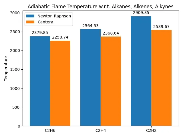
Figure 3.
It can be seen that the Adiabatic flame temperature is obtained from cantera is lower than the one obtained using NR method. It can be seen that as we move from Alkane to Alkyne the Adiabatic flame temperature obtained increase. This is because there are less number of molecules present in product formed and thus not require addition heat to raise the temperature.
4. Adiabatic flame temperature variation with respect to number of Carbon atom chains :
The hydrocarbon used are Methane, Ethane and Propane. The code for Adiabatic flame temperature is as follows:
import matplotlib.pyplot as plt
import numpy as np
import math

def h(T, coeff):

	R=8.314 #J/mol-K
	a1=coeff[0]
	a2=coeff[1]
	a3=coeff[2]
	a4=coeff[3]
	a5=coeff[4]
	a6=coeff[5]

	return (a1*T + a2*(pow(T,2)/2) + a3*(pow(T,3)/3) + a4*(pow(T,4)/4) + a5*(pow(T,5)/5) + a6)*R

ch4_coeffs_l = [5.14987613E+00, -1.36709788E-02, 4.91800599E-05, -4.84743026E-08, 1.66693956E-11, -1.02466476E+04, -4.64130376E+00]
c2h6_coeffs_l = [4.29142492E+00, -5.50154270E-03, 5.99438288E-05, -7.08466285E-08, 2.68685771E-11, -1.15222055E+04, 2.66682316E+00]
c3h8_coeffs_l = [0.93355381E+00, 0.26424579E-01, 0.61059727E-05, -0.21977499E-07, 0.95149253E-11, -0.13958520E+05, 0.19201691E+02]
o2_coeffs_l = [3.78245636E+00, -2.99673416E-03, 9.84730201E-06, -9.68129509E-09, 3.24372837E-12, -1.06394356E+03, 3.65767573E+00]
n2_coeffs_h = [0.02926640E+02, 0.14879768E-02, -0.05684760E-05, 0.10097038E-09, -0.06753351E-13, -0.09227977E+04, 0.05980528E+02]
n2_coeffs_l = [0.03298677E+02, 0.14082404E-02, -0.03963222E-04, 0.05641515E-07, -0.02444854E-10, -0.10208999E+04, 0.03950372E+02]
co2_coeffs_h = [3.85746029E+00, 4.41437026E-03, -2.21481404E-06, 5.23490188E-10, -4.72084164E-14, -4.87591660E+04, 2.27163806E+00]
h20_coeffs_h = [3.03399249E+00, 2.17691804E-03, -1.64072518E-07, -9.70419870E-11, 1.68200992E-14, -3.00042971E+04, 4.96677010E+00]

def f(T,n):
	#Product
	h_co2_p=h(T,co2_coeffs_h)
	h_h2o_p=h(T,h20_coeffs_h)
	h_n2_p=h(T,n2_coeffs_h)

	#Reactant
	Tstd=298.15
	h_o2_r=h(Tstd,o2_coeffs_l)
	h_n2_r=h(Tstd,n2_coeffs_l)
	h_ch4_r=h(Tstd,ch4_coeffs_l)
	h_c2h6_r=h(Tstd,c2h6_coeffs_l)
	h_c3h8_r=h(Tstd,c3h8_coeffs_l)

	if n==1:
		h_products=h_co2_p + 2*h_h2o_p + 7.52*h_n2_p
		h_reactants=h_ch4_r+2*h_o2_r+7.52*h_n2_r
	elif n==2:
		h_products=2*h_co2_p + 3*h_h2o_p + 13.16*h_n2_p
		h_reactants=h_c2h6_r+3.5*h_o2_r+13.16*h_n2_r
	elif n==3:
		h_products=3*h_co2_p + 4*h_h2o_p + 18.8*h_n2_p
		h_reactants=h_c3h8_r+5*h_o2_r+18.8*h_n2_r

	return h_products-h_reactants

def fprime(T,n):
	return (f(T+1e-06,n)-f(T,n))/1e-06

n=np.linspace(1,3,num=3)
fuels=['CH4','C2H6','C3H8']
l=len(n)
tol=1e-06
T_guess =np.ones(l)*1500
ct=np.zeros(l)
alpha=0.5

for i in range(l):
	while (abs(f(T_guess[i],n[i]))>tol):
		T_guess[i]=T_guess[i] - alpha*(f(T_guess[i],n[i])/fprime(T_guess[i],n[i]))
		ct[i]=ct[i]+1

print(ct)
print(T_guess)

T_ct=np.zeros(l)
#Cantera
import cantera as ct
for i in range(l):
	gas=ct.Solution('gri30.xml')
	if n[i]==1:
		n_o2=2
		n_n2=7.52
	elif n[i]==2:
		n_o2=3.5
		n_n2=13.16
	elif n[i]==3:
		n_o2=5
		n_n2=18.8

	gas.TPX=298.15,101325,{fuels[i]:1,'O2':n_o2,'N2':n_n2}
	gas.equilibrate('HP','auto')
	T_ct[i]=gas.T

print(T_ct)

x = np.arange(l)  # the label locations
width = 0.4  # the width of the bars

fig, ax = plt.subplots()
rects1 = ax.bar(x - width/2, T_guess, width, label='Newton Raphson')
rects2 = ax.bar(x + width/2, T_ct, width, label='Cantera')

# Add some text for labels, title and custom x-axis tick labels, etc.
ax.set_ylabel('Temperature')
ax.set_title('Adiabatic Flame Temperature w.r.t. Methane, Ethane, Propane')
ax.set_xticks(x, fuels)
ax.legend()

ax.bar_label(rects1, padding=3)
ax.bar_label(rects2, padding=3)

fig.tight_layout()

plt.show()
The plot obtained from the code can be seen in the figure 4.
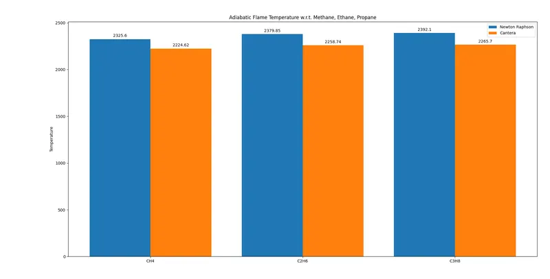
Figure 4.
In this plot it can be seen that as the number of carbon atom increases the AFT slightly increases also. This is because as the number of carbon atom increases the fuel increases leading to increase in AFT.