Week 3 - Adiabatic Flame Temperature calculation
Adiabatic Flame Temperature calculation
Introduction
If no heat is lost in the process of combustion, the temperature of the combustion products is known as the Adiabatic Flame Temperature (AFT). As a rule of thumb, more the combustion products, much energy is distributed among the particles and temperature is relatively low as compared to less product reactions. Temperature can also get influenced by mixture of inert materials in fuel. Often in the case where inert material is used with the fuels, the temperature is less.
Objective
Present study investigates, the effect of various hydrocarbons on AFT. Also, the effect of equivalence ratio on temperature raise will be investigated.
Introductory approach to Cantera module has also been used to compare the results with python. Here, our main objective is to see the variation in temperature with increased pollutants, as in the explicit calculation approach we won’t be considering each and every pollutant.
Python as a general programming language has been used in the simulation.
Outline
The study has been divided into four sections: -
- In the first section we discuss flame temperature variation with Equivalence ratio
- Discussion of effect of heat loss on the AFT
- Variation in AFT with different Hydrocarbons
- Variation in AFT with different no. of carbon atoms
The study has been done using python, a general programming language and Cantera Library.
Python Script
"""
Week 3 - Adiabatic Flame Temperature calculation - Solution
"""
# Importing the related modules
import matplotlib.pyplot as plt
import numpy as np
import cantera as cant
from numpy.core.shape_base import block


# For methane x = 1 and y = 4
x = 1
y = 4

# Constants
R = 8.314 # in J/mol-K

# Fuel Type
fuel_type = 0

# Polynomials Constants from NASA GRI-MECH
# Siffux "l" stands for low temperature and "h" stands for high temperature
c3h8_coeffs_l = [0.93355381E+00, 0.26424579E-01, 0.61059727E-05, -0.21977499E-07, 0.95149253E-11, -0.13958520E+05, 0.19201691E+02]
c2h6_coeffs_l = [4.29142492E+00, -5.50154270E-03, 5.99438288E-05, -7.08466285E-08, 2.68685771E-11, -1.15222055E+04, 2.66682316E+00]
c2h4_coeffs_l = [3.95920148E+00, -7.57052247E-03, 5.70990292E-05, -6.91588753E-08, 2.69884373E-11, 5.08977593E+03, 4.09733096E+00]
c2h2_coeffs_l = [8.08681094E-01, 2.33615629E-02, -3.55171815E-05, 2.80152437E-08, -8.50072974E-12, 2.64289807E+04, 1.39397051E+01]

ch4_coeffs_l = [5.14987613E+00, -1.36709788E-02, 4.91800599E-05, -4.84743026E-08, 1.66693956E-11, -1.02466476E+04, -4.64130376E+00]
o2_coeffs_l = [3.78245636E+00, -2.99673416E-03, 9.84730201E-06, -9.68129509E-09, 3.24372837E-12, -1.06394356E+03, 3.65767573E+00]
n2_coeffs_l = [0.03298677E+02, 0.14082404E-02, -0.03963222E-04, 0.05641515E-07, -0.02444854E-10, -0.10208999E+04, 0.03950372E+02]

n2_coeffs_h = [0.02926640E+02, 0.14879768E-02, -0.05684760E-05, 0.10097038E-09, -0.06753351E-13, -0.09227977E+04, 0.05980528E+02]
co2_coeffs_h = [3.85746029E+00, 4.41437026E-03, -2.21481404E-06, 5.23490188E-10, -4.72084164E-14, -4.87591660E+04, 2.27163806E+00]
h2o_coeffs_h = [3.03399249E+00, 2.17691804E-03, -1.64072518E-07, -9.70419870E-11, 1.68200992E-14, -3.00042971E+04, 4.96677010E+00]
o2_coeffs_h =  [3.78245636E+00, -2.99673416E-03, 9.84730201E-06, -9.68129509E-09, 3.24372837E-12, -1.06394356E+03, 3.65767573E+00]
co_coeffs_h = [2.71518561E+00, 2.06252743E-03, -9.98825771E-07, 2.30053008E-10, -2.03647716E-14, -1.41518724E+04, 7.81868772E+00]


# Enthalpy Calculation as per NASA Polynomials

def h(T, co_effs):

	a1 = co_effs[0]
	a2 = co_effs[1]
	a3 = co_effs[2]
	a4 = co_effs[3]
	a5 = co_effs[4]
	a6 = co_effs[5]

	return (a1 + a2*T/2 + a3*pow(T,2)/3 + a4*pow(T,3)/4 + a5*pow(T,4)/5 + a6/T)*R*T

# Reaction Enthalpy function polynomial without heat loss

def f(T):

	# Products At Temperature T

	h_co2_p = h(T, co2_coeffs_h)
	h_h2o_p = h(T, h2o_coeffs_h)
	h_n2_p = h(T, n2_coeffs_h)
	h_o2_p = h(T, o2_coeffs_h)
	h_co_p = h(T, co_coeffs_h)
	H_products = a*h_co2_p + b*h_h2o_p + c*h_n2_p + d*h_o2_p + e*h_co_p

	n_products = a + b + c + d + e
	nRT_products = n_products * R * T

	# Reactants At Standard Temperature

	T_std = 298.15
	h_ch4_r = h(T_std, ch4_coeffs_l)
	h_o2_r = h(T_std, o2_coeffs_l)
	h_n2_r = h(T_std, n2_coeffs_l)
	H_reactants = h_ch4_r + g*h_o2_r + 3.76*g*h_n2_r

	n_reactants = 1 + g + 3.76*g
	nRT_reactants = n_reactants * R * T_std

	return (H_products - H_reactants) - (nRT_products - nRT_reactants)

# Numerical Derivative Calculator

def fprime(func, arg):
	return (func(arg+1e-6) - func(arg)) / 1e-6

# Reaction Enthalpy function polynomial with heat loss

def f_hloss(T):
    # Products At Temperature T

    h_co2_p = h(T, co2_coeffs_h)
    h_h2o_p = h(T, h2o_coeffs_h)
    h_n2_p = h(T, n2_coeffs_h)
    h_o2_p = h(T, o2_coeffs_h)
    h_co_p = h(T, co_coeffs_h)
    H_products = a*h_co2_p + b*h_h2o_p + c*h_n2_p + d*h_o2_p + e*h_co_p

	# Products At Standard Temperature
    T_std = 298.15
    h_co2_p_std = h(T_std, co2_coeffs_h)
    h_h2o_p_std = h(T_std, h2o_coeffs_h)
    h_n2_p_std = h(T_std, n2_coeffs_h)
    h_o2_p_std = h(T_std, o2_coeffs_h)
    h_co_p_std = h(T_std, co_coeffs_h)
    H_products_std = a*h_co2_p_std + b*h_h2o_p_std + c*h_n2_p_std + d*h_o2_p_std + e*h_co_p_std

    # Reactants At Standard Temperature
    if fuel_type == 0:
        h_fuel = h(T_std, ch4_coeffs_l)
    if fuel_type == 1:
        h_fuel = h(T_std, c2h6_coeffs_l)
    if fuel_type == 2:
        h_fuel = h(T_std, c2h4_coeffs_l)
    if fuel_type == 3:
        h_fuel = h(T_std, c2h2_coeffs_l)
    if fuel_type == 4:
        h_fuel = h(T_std, c3h8_coeffs_l)

    # h_ch4_r = h(T_std, ch4_coeffs_l)
    h_o2_r = h(T_std, o2_coeffs_l)
    h_n2_r = h(T_std, n2_coeffs_l)
    H_reactants = h_fuel + g*h_o2_r + 3.76*g*h_n2_r

    # Lower Heating Value

    LHV = H_reactants - H_products_std

    return H_products - H_reactants + (H_loss * LHV)

def labeling(rects):

    for rect in rects:
        height = rect.get_height()
        ax.text(rect.get_x() + rect.get_width()/2., height, '%0.3f K' % float(height), ha='center', va='bottom')

"""
	Let the General Equation for combustion of Hydrocarbon:
		CxHy + g(O2 + 3.76N2) = aCO2 + bH2O + cN2 + dO2 + eCO
        For Methane,
		x = 1; y = 4; ar = x + y/4; g = ar * (1/fi)

	Stoichiometric Equation (fi = 1):
		CxHy + ar(O2 + 3.76N2) = xCO2 + (y/2)H2O + 3.76(x + y/4)N2
	Lean Mixture Equation (fi < 1):
		CxHy + ar(1/fi)(O2 + 3.76N2) = xCO2 + (y/2)H2O + 3.76(ar/fi)N2 + ar((1/fi)-1)O2
	Rich Mixture Equation (fi > 1):
		CxHy + ar(1/fi)(O2 + 3.76N2) = ((ar/2fi) - x - y/2)CO2 + (y/2)H2O + 3.76(ar/fi)N2 + (2x + (y/2) - (ar/2fi))CO
"""

# 1. Adiabatic flame temperature variation with Equivalence ratio (In constant volume-chamber) :

# Initial Guess of temeprature has been set as 1500 K


# Array variable for Storing AFT temperature with python approach
temp_python = []
# Lower limit of the Equivalence ratio
fiLowerLimit = 0.1
# Upper limit of the Equivalence ratio
fiUpperLimit = 2
# Difference over which equivalence ratio has been advanced
diff = 0.1
# Numpy module has been used to create the Equivalence ratio array
fi = np.arange(fiLowerLimit, fiUpperLimit + diff, diff)

# Loop for calculating the coefficients
for i in range (0, len(fi)):

	if (fi[i] == 1):
		ar = x + y/4
		g = ar
		a = x
		b = y/2
		c = 3.76 * ar
		d = 0
		e = 0

	if (fi[i] < 1):
		ar = x + y/4
		g = ar * (1/fi[i])
		a = x
		b = y/2
		c = 3.76 * ar * (1/fi[i])
		d = ar * ((1/fi[i])-1)
		e = 0

	if (fi[i] > 1):
		ar = x + y/4
		g = ar * (1/fi[i])
		a = (2*ar/fi[i]) - x - y/2
		b = y/2
		c = 3.76 * ar * (1/fi[i])
		d = 0
		e = 2*x + y/2 - (2*ar)/fi[i]


	temperature_temp = 1500
	tol = 1e-6
	alpha = 0.2
	iter = 0

	while (abs(f(temperature_temp)) > tol):
		temperature_temp = temperature_temp - alpha * (f(temperature_temp) / fprime(f, temperature_temp))
		iter = iter + 1

	temp_python.append(temperature_temp)

# Solution using cantera

gas = cant.Solution('gri30.xml')
# Array variable for Storing AFT temperature with Cantera approach
temp_cant = []

for i in range(0, len(fi)):

	n_total = 1 + (ar/fi[i]) + 3.76*(ar/fi[i])
	n_ch4 = 1/n_total
	n_o2 = (ar/fi[i])/n_total
	n_n2 = (3.76*(ar/fi[i]))/n_total

	gas.TPX = 298.15, 101325, {'CH4':n_ch4, 'O2':n_o2, 'N2':n_n2}
	gas.equilibrate('UV', 'auto')
	temp_cant.append(gas.T)


fig1 = plt.figure()

# Variation in the results from cantera and explicit python code
plt.plot(fi, temp_cant, '-o', color = 'green', label = 'Cantera-Solution')
plt.plot(fi, temp_python, '-o', color = 'red', label = 'Python-Solution')


plt.title('1. Effect of Variation in Equivalence Ratio on Adiabatic Flame Temperature \n' + 'Constant Volume Chamber')
plt.xlabel('Varying Equivalence Ratio, $Φ$')
plt.ylabel('Adiabatic Flame Temperature ($K$)')

plt.legend()
plt.xticks(np.arange(0, 2.1, 0.2))
plt.yticks(np.arange(400, 3000, 200))
plt.show(block=False)


# 2. Adiabatic flame temperature variation with Heat loss (In constant pressure-chamber) :


H_loss_fraction_array = []
temp_aft = []
# As given Heat Loss fration to be 0.35
H_loss = 0
H_loss_max = 1

# Since equivalence ratio is 1
ar = x + y/4
g = ar
a = x
b = y/2
c = 3.76 * ar
d = 0
e = 0


temperature_temp = 1500
tol = 1e-6
# As given in the problem alpha shoulb be 1
alpha = 1
iter = 0

while (H_loss <= H_loss_max):
    while (abs(f_hloss(temperature_temp)) > tol):
        temperature_temp = temperature_temp - (alpha * (f_hloss(temperature_temp) / fprime(f_hloss,temperature_temp)))
        iter = iter + 1


    H_loss_fraction_array.append(H_loss)
    temp_aft.append(temperature_temp)
    if H_loss == 0.35:
        print("AFT at Heat Loss of 35% =", temperature_temp)
    H_loss = round(H_loss + 0.05,2)


# Plotting the results obtained from Python
fig2 = plt.figure()

plt.plot(H_loss_fraction_array, temp_aft, '-o', color = 'red')
plt.ylim(0,2500)
plt.xticks(np.arange(0, 1.1, 0.1))
plt.yticks(np.arange(0, 2500, 200))
plt.xlabel('Heat Loss Fraction')
plt.ylabel('Adiabatic Flame Temperature (K)')
plt.title('Effect of Heat Loss Fraction on the AFT \n'
			+ 'in Constant Pressure Chamber')

plt.show(block=False)


# 3. Adiabatic flame temperature variation with respect to Alkane, Alkene, Alkyne :


# Calculating the temperature and storing the values

temp_aft = []
H_loss = 0

for fuel_type in range (1, 4):
    phi_py = 1
    H_loss = 0.35

    if fuel_type == 1:
        x = 2
        y = 6
    elif fuel_type == 2:
        x = 2
        y = 4
    elif fuel_type == 3:
        x = 2
        y = 2

    ar = x + y/4
    g = ar
    a = x
    b = y/2
    c = 3.76 * ar
    d = 0
    e = 0

    T_guess = 1500

    tol = 1e-6
    alpha = 0.2
    ct = 0

    while (abs(f_hloss(T_guess)) > tol):
        T_guess = T_guess - alpha * (f_hloss(T_guess) / fprime(f_hloss,T_guess))
        ct = ct + 1

    temp_aft.append(T_guess)

x_bar = ['Ethane', 'Ethene', 'Ethyne']
x_pos = [i for i, _ in enumerate(x_bar)]

fig, ax = plt.subplots()
bars = ax.bar(x_pos, temp_aft)
plt.ylim(1700, 2100)
plt.xlabel("Types of Hydrocarbon")
plt.ylabel("Adiabatic Flame Temperature (K)")
plt.title("Variation of Adiabatic Flame Temperature \n for different Hydrocarbonsn")
plt.xticks(x_pos, x_bar)

labeling(bars)

plt.show(block=False)


# 4. Adiabatic flame temperature variation with respect to a number of Carbon atom chains :

# Variable for storing AFT
temp_aft = []
# Heat loss has been 0
H_loss = 0

for fuel_type in [0, 1, 4]:
    if fuel_type == 0:
        x = 1
        y = 4
    elif fuel_type == 1:
        x = 2
        y = 6
    elif fuel_type == 4:
        x = 3
        y = 8

    ar = x + y/4
    g = ar
    a = x
    b = y/2
    c = 3.76 * ar
    d = 0
    e = 0

    T_guess = 1500
    tol = 1e-6
    alpha = 0.2
    iter = 0

    while (abs(f_hloss(T_guess)) > tol):
        T_guess = T_guess - alpha * (f_hloss(T_guess) / fprime(f_hloss, T_guess))
        iter = iter + 1

    temp_aft.append(T_guess)

# Plotting the results obtained from Python


x_bar = ['Methane', 'Ethane', 'Propane']
x_pos = [i for i, _ in enumerate(x_bar)]

fig, ax = plt.subplots()
bars = ax.bar(x_pos, temp_aft)
plt.ylim(2300, 2400)
plt.xlabel("Type of Alkane (Carbon atom variation)")
plt.ylabel("Adiabatic Flame Temperature (K)")
plt.title("Adiabatic Flame Temperature For Different Alkanes")
plt.xticks(x_pos, x_bar)

labeling(bars)

plt.show()
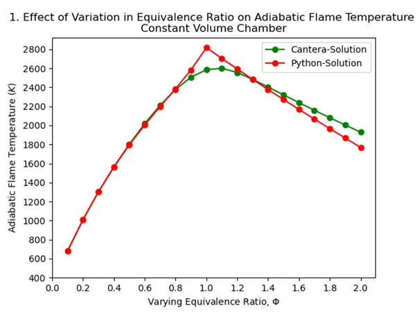
Adiabatic flame temperature variation with Equivalence ratio (In constant volume-chamber)
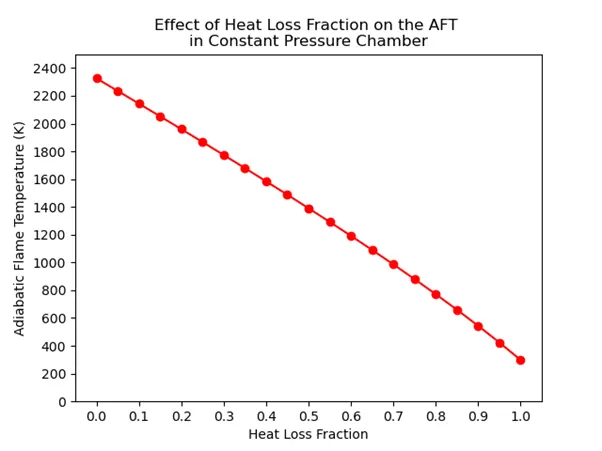
Adiabatic flame temperature variation with Heat loss (In constant pressure-chamber)
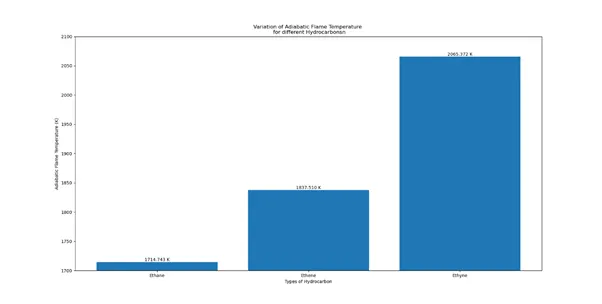
Adiabatic flame temperature variation with respect to Alkane, Alkene, Alkyne
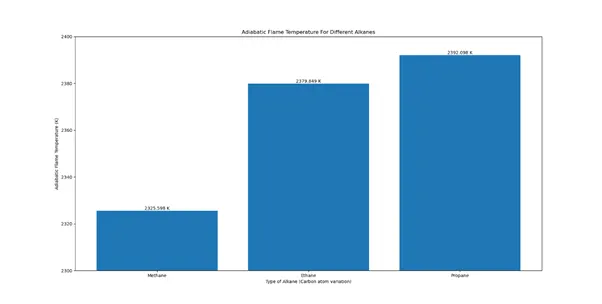
Adiabatic flame temperature variation with respect to a number of Carbon atom chains
Conclusions:
AFT calculated from python as well as using Cantera library has similar corelation, till around 0.8 Equivalence ratio. After that, our python script slightly over shoots the values. This can be corelated from the fact that we have not included all the pollutants that has the potential to form in the given chemical reaction. While, Cantera library has rich resource of the reactions governing the combustion process.
As can be seen from the plot, The increase in Heat loss fraction has led to the decrease in AFT. Also, at Heat Loss fraction of 0.35, the calculated AFT has a value of around 1679 K as per out python script.
The increase in AFT with Heavier fuels. This can be corelated with the increased bonding between the elements.
As in the previous case, AFT has increased with the increase in Carbon atoms. The trend temperature elevation can be seen differing from the previous case, which can be attributed to difference in bonding.