Week 3 - Adiabatic Flame Temperature calculation

Adiabatic Flame Temperature Calculation

• Aim :

1. Plotting the effect of equivalence ratio on Adiabatic Flame Temperature of Methane in a constant volume chamber with N2 present.
2. Calculate Adiabatic Flame Temperature with varying heat loss.
3. Calculate Adiabatic flame temperature variation with respect to Alkane, Alkene, Alkyne.
4. Calculate Adiabatic flame temperature variation with respect to a number of Carbon atom chains.

• Theory :

Combustion Reaction : A combustion reaction is a reaction in which a substance reacts with oxygen gas, releasing energy in the form of light and heat. Combustion reactions must involve O2 as one reactant. The combustion of hydrogen gas produces water vapor. Many combustion reactions occur with a hydrocarbon, a compound made up solely of carbon and hydrogen. The products of the combustion of hydrocarbons are carbon dioxide and water. Many hydrocarbons are used as fuel because their combustion releases very large amounts of heat energy. propane is a gaseous hydrocarbon that is commonly used as the fuel source in gas grills.

Equivalence Ratio : The equivalence ratio (`phi`) is defined as the ratio of the actual fuel/air ratio to the stoichiometric fuel/air ratio. Stoichiometric combustion occurs when all the oxygen is consumed in the reaction, and there is no molecular oxygen(O2) in the products.If the equivalence ratio is equal to one, the combustion is stoichiometric. If it is < 1, the combustion is lean with excess air, and if it is >1, the combustion is rich with incomplete combustion.

Adiabatic Flame Temperature : The adiabatic flame temperature is one that occurs when the combustion chamber is well insulated with no heat losses (adiabatic conditions). The peak adiabatic flame temperature occurs at around Φ = 1 in an ideally insulated combustion chamber. The constant volume adiabatic flame temperature is the temperature that results from a complete combustion process that occurs without any work, heat transfer or changes in kinetic or potential energy. Its temperature is higher than the constant pressure process because no energy is utilized to change the volume of the system (i.e., generate work).

Enthalpy calculation using NASA polynomials : NASA came up with polynomials that can be used to evaluate thermodynamic properties such as Cp, H, and S. They have documented the coefficients that are required to evaluate these polynomials for 1000+ species.

Enthalpy is calculated using NASA polynomials, which is given by

`H/(RT) = a_1 + a_2 T /2 + a_3 T^2 /3 + a_4 T^3 /4 + a_5 T^4 /5 + a_6/T`

where H = enthalpy, R = universal gas constant, T = temperature.

Newton Raphson method : The Newton-Raphson method (also known as Newton's method) is a way to quickly find a good approximation for the root of a real-valued function f(x) = 0. It uses the idea that a continuous and differentiable function can be approximated by a straight line tangent to it. Suppose you need to find the root of a continuous, differentiable function f(x), and you know the root you are looking for is near the point x = `x_0`​. Then Newton's method tells us that a better approximation for the root is

`x_1 = x_0 -[ f(x_0)]/[f'(x_0)]`

Cantera : Cantera is an open-source suite of tools for problems involving chemical kinetics, thermodynamics, and transport processes. Cantera was originally written and developed by Prof. Dave Goodwin . It is written in C++ and can be used from C++, Python, Matlab and Fortran.

Cantera can be imported using the command 'import cantera as ct'.​ Cantera has inbuilt all values of NASA polynomials for different species. The command 'gas = ct.Solution('gri30.xml')' will help us define a class as gas. 'gas.TPX' and 'gas.equilibriate' will help us calculate AFT of different species as we like.

1. Plotting the effect of equivalence ratio on Adiabatic Flame Temperature of Methane in a constant volume chamber with N2 present.

For lean mixture i.e `phi`< 1,

`CH_4 + 2/phi *(O_2 + 3.76 N_2) = CO_2 + 2H_2O+(2/phi-2)O_2 +7.52/phiN_2`

For rich mixture i.e `phi`> 1

`CH_4+2/phi(O_2 +3.76N_2)=(4/phi -3)CO_2 + 2H_2O+(4-4/phi)CO + 7.52/phiN_2`

"""
 Adiabatic Flame Temperature variation with Equivalence ratio 
 """
import matplotlib.pyplot as plt 

# CH4 + (2/phi)*(O2 + 3.76N2) = CO2 + 2H2O + (7.52/phi)N2 + (2/phi - 2)O2 -----Stoichometric equation for lean mixture

# CH4 + (2/phi)*(O2 + 3.76N2) = (4/phi- 3)CO2 + 2H2O + (7.52/phi)N2 + (4 - 4/phi)CO -----Stoichometric equation for rich mixture


def h(T,coeffs):
 	R = 8.314 # J/mol*K

 	a1 = coeffs[0]
 	a2 = coeffs[1]
 	a3 = coeffs[2]
 	a4 = coeffs[3]
 	a5 = coeffs[4]
 	a6 = coeffs[5]

 	return (a1 + a2/2*T + a3/3*pow(T,2) + a4/4*pow(T,3) + a5/5*pow(T,4) + a6/T)*R*T

"""
 Defining coefficients of reactants
 """

ch4_coeefs_r = [5.14987613E+00, -1.36709788E-02, 4.91800599E-05, -4.84743026E-08, 1.66693956E-11,-1.02466476E+04, -4.64130376E+00]

o2_coeffs_r = [3.78245636E+00, -2.99673416E-03, 9.84730201E-06,  -9.68129509E-09, 3.24372837E-12, -1.06394356E+03, 3.65767573E+00]

n2_coeffs_r = [0.03298677E+02, 0.14082404E-02, -0.03963222E-04, 0.05641515E-07, -0.02444854E-10, -0.10208999E+04, 0.03950372E+02]

"""
Defining coefficients of product
"""
co2_coeffs_p = [3.85746029E+00, 4.41437026E-03, -2.21481404E-06, 5.23490188E-10, -4.72084164E-14, -4.87591660E+04, 2.27163806E+00]

h2o_coeffs_p = [3.03399249E+00, 2.17691804E-03, -1.64072518E-07, -9.70419870E-11, 1.68200992E-14, -3.00042971E+04, 4.96677010E+00]

n2_coeffs_p = [0.02926640E+02, 0.14879768E-02, -0.05684760E-05, 0.10097038E-09, -0.06753351E-13, -0.09227977E+04, 0.05980528E+02]

o2_coeffs_p = [3.28253784E+00, 1.48308754E-03, -7.57966669E-07, 2.09470555E-10, -2.16717794E-14, -1.08845772E+03, 5.45323129E+00]

co_coeffs_p = [2.71518561E+00, 2.06252743E-03, -9.98825771E-07, 2.30053008E-10, -2.03647716E-14, -1.41518724E+04, 7.81868772E+00]

"""
Defining matrix for phi
"""
phi_value = []

"""
Defining matrix for AFT
"""
AFT_value = []

"""
Defining a function to calculate enthalpy of products
"""

def f(T):
	h_CO2_p = h(T,co2_coeffs_p)
	h_H2O_p = h(T,h2o_coeffs_p)
	h_N2_p = h(T,n2_coeffs_p)
	h_O2_p = h(T,o2_coeffs_p)
	h_CO_p = h(T,co_coeffs_p)

	if phi <= 1:
		h_products = h_CO2_p + (2*h_H2O_p) + (7.52/phi*h_N2_p) + (((2/phi)-2)*h_O2_p)

		n_p = 1 + 2 + (7.52/phi) + ((2/phi)-2)

	else:
		h_products = ((4/phi)-3)*h_CO2_p + (2*h_H2O_p) + (7.52/phi*h_N2_p) + ((4-4/phi)*h_CO_p)

		n_p = ((4/phi)-3) + 2 + (7.52/phi) + (4-(4/phi))

	return (h_products - h_reactants + 8.314*((n_r*T_std) - (n_p*T)))

"""
defining fprime
"""

def fprime(T):
	return (f(T+1e-6) - f(T))/(1e-6)

for i in range (1,18):
	phi = i/10

	phi_value.append(phi)

	"""
	Calculating enthalpy of reactants
	"""

	T_std = 298.15

	h_CH4_r = h(T_std,ch4_coeefs_r)
	h_O2_r = h(T_std,o2_coeffs_r)
	h_N2_r = h(T_std,n2_coeffs_r)




	h_reactants = (h_CH4_r*1) + (2/phi*h_O2_r) + (7.52/phi*h_N2_r)

	n_r = 1 + (2/phi) + (7.52/phi)

	tol = 1e-4 
	T_aft = 3000
	alpha = 0.2

	while(abs(f(T_aft)) > tol):

		T_aft = T_aft - (alpha*f(T_aft)/fprime(T_aft))

	AFT_value.append(T_aft)



"""
AFT using cantera
"""

import cantera as ct
import matplotlib.pyplot as plt


gas = ct.Solution('gri30.xml')

phi_cantera = []

AFT_cantera = []



for i in range(1,18):

	phi = i/10

	phi_cantera.append(phi)

	gas.TPX = 298.15,101325,{'CH4':1, 'O2':2/phi, 'N2':7.52/phi}

	gas.equilibrate('UV', 'auto')

	AFT_cantera.append(gas.T)



print(AFT_value)
print(AFT_cantera)
print(phi_value)
print(phi_cantera)
plt.plot(phi_value,AFT_value,color='blue',label='python')
plt.plot(phi_cantera,AFT_cantera,color='red',label='cantera')
plt.xlabel('Phi values')
plt.ylabel('AFT values in K')
plt.title('AFT vs Phi')
plt.legend()
plt.show()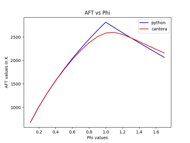

Highest value of Adiabatic flame temperature is obtained near `phi` = 1.0 using python and `phi` = 1.1 using cantera. Two curves have slight variation as cantera considers more number of species at product side. Overall the two curves match showing the python code and AFT values are verified.

2. Calculating Adiabatic Flame Temperature with varying heat loss.

A. Effect of heat loss factor on AFT

Q is the heat loss factor, which can vary from 0 to 1. Meaning if the heat loss percentage is 50% then Q = 0.5.

Heat loss = Q. H_max, where H_max is maximum enthalpy

H_max = H_reactants - H_products(lower range)

where, H_reactants = enthalpy of reactants

H_products = enthalpy of products

"""
Determining AFT of CH4 with enthalpy loss
 """
import matplotlib.pyplot as plt 
import numpy as np

# CH4 + 2(O2 + 3.76N2) = CO2 + 2H2O + 7.52N2 ----- Stoichometric equation for combustion of CH4

def h(T,coeffs):
 	R = 8.314 # J/mol*K

 	a1 = coeffs[0]
 	a2 = coeffs[1]
 	a3 = coeffs[2]
 	a4 = coeffs[3]
 	a5 = coeffs[4]
 	a6 = coeffs[5]

 	return (a1 + a2/2*T + a3/3*pow(T,2) + a4/4*pow(T,3) + a5/5*pow(T,4) + a6/T)*R*T


"""
 Defining coefficients of reactants
 """

ch4_coeefs_r = [5.14987613E+00, -1.36709788E-02, 4.91800599E-05, -4.84743026E-08, 1.66693956E-11,-1.02466476E+04, -4.64130376E+00]

o2_coeffs_r = [3.78245636E+00, -2.99673416E-03, 9.84730201E-06,  -9.68129509E-09, 3.24372837E-12, -1.06394356E+03, 3.65767573E+00]

n2_coeffs_r = [0.03298677E+02, 0.14082404E-02, -0.03963222E-04, 0.05641515E-07, -0.02444854E-10, -0.10208999E+04, 0.03950372E+02]

"""
Defining coefficients of product
"""

co2_coeffs_p = [3.85746029E+00, 4.41437026E-03, -2.21481404E-06, 5.23490188E-10, -4.72084164E-14, -4.87591660E+04, 2.27163806E+00]

h2o_coeffs_p = [3.03399249E+00, 2.17691804E-03, -1.64072518E-07, -9.70419870E-11, 1.68200992E-14, -3.00042971E+04, 4.96677010E+00]

n2_coeffs_p = [0.02926640E+02, 0.14879768E-02, -0.05684760E-05, 0.10097038E-09, -0.06753351E-13, -0.09227977E+04, 0.05980528E+02]

"""
Defining coefficients for products at low temp. range
"""

co2_coeffs_l = [2.35677352E+00, 8.98459677E-03, -7.12356269E-06, 2.45919022E-09, -1.43699548E-13, -4.83719697E+04, 9.90105222E+00]

h2o_coeffs_l = [4.19864056E+00, -2.03643410E-03, 6.52040211E-06, -5.48797062E-09, 1.77197817E-12, -3.02937267E+04, -8.49032208E-01]

n2_coeffs_l = [0.03298677E+02, 0.14082404E-02, -0.03963222E-04, 0.05641515E-07, -0.02444854E-10, -0.10208999E+04, 0.03950372E+02]

"""
Calculating enthalpy of reactants
"""

T_std = 298.15

h_CH4_r = h(T_std,ch4_coeefs_r)
h_O2_r = h(T_std,o2_coeffs_r)
h_N2_r = h(T_std,n2_coeffs_r)

h_reactants = (h_CH4_r*1) + (2*h_O2_r) + (7.52*h_N2_r)

"""
Defining a function to calculate enthalpy of products
"""

def f(T,Q):
	h_CO2_p = h(T,co2_coeffs_p)
	h_H2O_p = h(T,h2o_coeffs_p)
	h_N2_p = h(T,n2_coeffs_p)

	h_products = h_CO2_p + 2*h_H2O_p + 7.52*h_N2_p

	h_max = h_reactants - h(T_std,co2_coeffs_l) - (2*h(T_std,h2o_coeffs_l)) - (7.52*h(T_std,n2_coeffs_l))

	return h_products - h_reactants + Q*h_max

def fprime(T,Q):
	return (f((T+1e-6),Q) - f(T,Q))/(1e-6)

tol = 1e-4
T_aft = 3000
alpha = 0.2

AFT_value = []

Q = np.linspace(0,1,20)

for i in Q:


	while(abs(f(T_aft,i)) > tol):

		T_aft = T_aft - (alpha*f(T_aft,i)/fprime(T_aft,i))

	AFT_value.append(T_aft)
		
plt.plot(Q,AFT_value,'-*',color = 'red')
plt.xlabel('Heat loss factor')
plt.ylabel('AFT values in K')
plt.title('AFT variation with heat loss')
plt.grid('on')


print(AFT_value)
plt.show()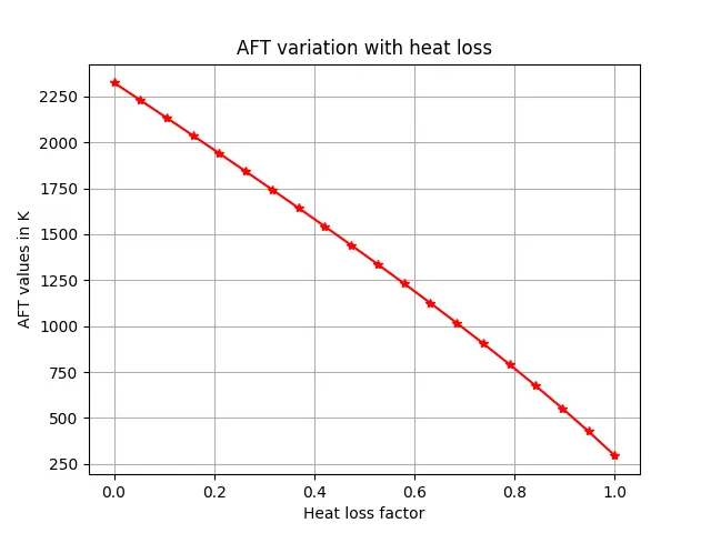

It can be observed the Adibatic flame temperature lowers linearly as the heat loss factor increases. Maximum heat loss occurs when heat loss factor = 1.

B. Calculating AFT with heat loss of 35%

Q = 0.35

"""
Determining AFT of CH4 with enthalpy loss
 """
import matplotlib.pyplot as plt 

# CH4 + 2(O2 + 3.76N2) = CO2 + 2H2O + 7.52N2 ----- Stoichometric equation for combustion of CH4

def h(T,coeffs):
 	R = 8.314 # J/mol*K

 	a1 = coeffs[0]
 	a2 = coeffs[1]
 	a3 = coeffs[2]
 	a4 = coeffs[3]
 	a5 = coeffs[4]
 	a6 = coeffs[5]

 	return (a1 + a2/2*T + a3/3*pow(T,2) + a4/4*pow(T,3) + a5/5*pow(T,4) + a6/T)*R*T


"""
 Defining coefficients of reactants
 """

ch4_coeefs_r = [5.14987613E+00, -1.36709788E-02, 4.91800599E-05, -4.84743026E-08, 1.66693956E-11,-1.02466476E+04, -4.64130376E+00]

o2_coeffs_r = [3.78245636E+00, -2.99673416E-03, 9.84730201E-06,  -9.68129509E-09, 3.24372837E-12, -1.06394356E+03, 3.65767573E+00]

n2_coeffs_r = [0.03298677E+02, 0.14082404E-02, -0.03963222E-04, 0.05641515E-07, -0.02444854E-10, -0.10208999E+04, 0.03950372E+02]

"""
Defining coefficients of product
"""

co2_coeffs_p = [3.85746029E+00, 4.41437026E-03, -2.21481404E-06, 5.23490188E-10, -4.72084164E-14, -4.87591660E+04, 2.27163806E+00]

h2o_coeffs_p = [3.03399249E+00, 2.17691804E-03, -1.64072518E-07, -9.70419870E-11, 1.68200992E-14, -3.00042971E+04, 4.96677010E+00]

n2_coeffs_p = [0.02926640E+02, 0.14879768E-02, -0.05684760E-05, 0.10097038E-09, -0.06753351E-13, -0.09227977E+04, 0.05980528E+02]

"""
Defining coefficients for products at low temp. range
"""

co2_coeffs_l = [2.35677352E+00, 8.98459677E-03, -7.12356269E-06, 2.45919022E-09, -1.43699548E-13, -4.83719697E+04, 9.90105222E+00]

h2o_coeffs_l = [4.19864056E+00, -2.03643410E-03, 6.52040211E-06, -5.48797062E-09, 1.77197817E-12, -3.02937267E+04, -8.49032208E-01]

n2_coeffs_l = [0.03298677E+02, 0.14082404E-02, -0.03963222E-04, 0.05641515E-07, -0.02444854E-10, -0.10208999E+04, 0.03950372E+02]

"""
Calculating enthalpy of reactants
"""

T_std = 298.15

h_CH4_r = h(T_std,ch4_coeefs_r)
h_O2_r = h(T_std,o2_coeffs_r)
h_N2_r = h(T_std,n2_coeffs_r)

h_reactants = (h_CH4_r*1) + (2*h_O2_r) + (7.52*h_N2_r)

"""
Defining a function to calculate enthalpy of products
"""

def f(T):
	h_CO2_p = h(T,co2_coeffs_p)
	h_H2O_p = h(T,h2o_coeffs_p)
	h_N2_p = h(T,n2_coeffs_p)

	h_products = h_CO2_p + 2*h_H2O_p + 7.52*h_N2_p

	h_max = h_reactants - h(T_std,co2_coeffs_l) - (2*h(T_std,h2o_coeffs_l)) - (7.52*h(T_std,n2_coeffs_l))

	return h_products - h_reactants + 0.35*h_max

def fprime(T):
	return (f(T+1e-6) - f(T))/(1e-6)

tol = 1e-4
T_aft = 3000
alpha = 0.2
iter = 0

while(abs(f(T_aft)) > tol):

		T_aft = T_aft - (alpha*f(T_aft)/fprime(T_aft))

		iter = iter +1
		plt.plot(iter,T_aft,'.',color = 'red')
		plt.xlabel('No. of Iterations')
		plt.ylabel('AFT values in K')
		plt.title('AFT variation with')



print(T_aft)
print(iter)
plt.show()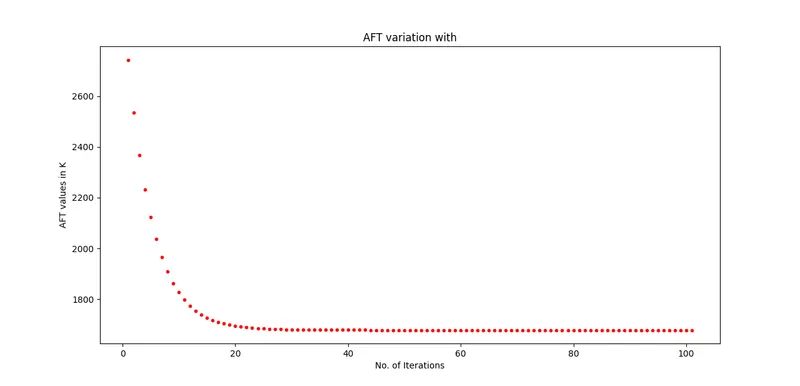

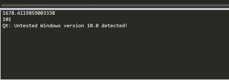
As observed through the plot, the value of AFT remains closer to the final value for most of the iterations. Also the value of AFT can be verified from previous case where AFT = 1643.39K when Q = 0.35, which is close to obtained value of AFT = 1678.41 K.

3. Adiabatic flame Temperature of Alkane, Alkene and Alkyne.

`C_2H_6 + 3.5(O_2 + 3.76N_2) = 2CO_2 + 3H_2O + 13.16N_2`

`C_2H_4 + 3(O_2 + 3.76N_2) = 2CO_2 + 2H_2O + 11.28N_2`

`C_2H_2 + 2.5(O_2 + 3.76N_2) = 2CO_2 + H_2O + 9.4N_2`

"""
AFT variation with respect to alkanes, alkenes, alkynes
"""
# C2H6 + 3.5(O2 + 3.76N2) = 2CO2 + 3H2O + 13.16N2 --- Stoichometric combustion of ethane

# C2H4 + 3(O2 + 3.76N2) = 2CO2 + 2H2O + 11.28N2 --- Stoichometric combustion of ethene

# C2H2 + 2.5(O2 + 3.76N2) = 2CO2 + H2O + 9.4N2 --- Stoichometric combustion of ethyne


import matplotlib.pyplot as plt 

def h(T,coeffs):
 	R = 8.314 # J/mol*K

 	a1 = coeffs[0]
 	a2 = coeffs[1]
 	a3 = coeffs[2]
 	a4 = coeffs[3]
 	a5 = coeffs[4]
 	a6 = coeffs[5]

 	return (a1 + a2/2*T + a3/3*pow(T,2) + a4/4*pow(T,3) + a5/5*pow(T,4) + a6/T)*R*T

"""
 Defining coefficients of reactants
 """

o2_coeffs_r = [3.78245636E+00, -2.99673416E-03, 9.84730201E-06,  -9.68129509E-09, 3.24372837E-12, -1.06394356E+03, 3.65767573E+00]

n2_coeffs_r = [0.03298677E+02, 0.14082404E-02, -0.03963222E-04, 0.05641515E-07, -0.02444854E-10, -0.10208999E+04, 0.03950372E+02]

c2h6_coeffs_r = [4.29142492E+00, -5.50154270E-03, 5.99438288E-05, -7.08466285E-08, 2.68685771E-11, -1.15222055E+04, 2.66682316E+00]

c2h4_coeffs_r = [3.95920148E+00, -7.57052247E-03, 5.70990292E-05, -6.91588753E-08, 2.69884373E-11, 5.08977593E+03, 4.09733096E+00]

c2h2_coeffs_r = [8.08681094E-01, 2.33615629E-02, -3.55171815E-05, 2.80152437E-08, -8.50072974E-12, 2.64289807E+04, 1.39397051E+01]

"""
Defining coefficients of product
"""

co2_coeffs_p = [3.85746029E+00, 4.41437026E-03, -2.21481404E-06, 5.23490188E-10, -4.72084164E-14, -4.87591660E+04, 2.27163806E+00]

h2o_coeffs_p = [3.03399249E+00, 2.17691804E-03, -1.64072518E-07, -9.70419870E-11, 1.68200992E-14, -3.00042971E+04, 4.96677010E+00]

n2_coeffs_p = [0.02926640E+02, 0.14879768E-02, -0.05684760E-05, 0.10097038E-09, -0.06753351E-13, -0.09227977E+04, 0.05980528E+02]

"""
Defining a matrix for AFT values
"""
AFT_value = []

"""
Defining a function to calculate AFT
"""
def f(T):

	"""
	Calculating enthalpy of reactants
	"""

	T_std = 298.15

	h_C2H6_r = h(T_std,c2h6_coeffs_r)
	h_C2H4_r = h(T_std,c2h4_coeffs_r)
	h_C2H2_r = h(T_std,c2h2_coeffs_r)
	h_O2_r = h(T_std,o2_coeffs_r)
	h_N2_r = h(T_std,n2_coeffs_r)

	"""
	calculating enthalpy ofproducts
	"""

	h_CO2_p = h(T,co2_coeffs_p)
	h_H2O_p = h(T,h2o_coeffs_p)
	h_N2_p = h(T,n2_coeffs_p)

	if c == 1:
		h_reactants = h_C2H6_r + 3.5*h_O2_r + 13.16*h_N2_r

		h_products = 2*h_CO2_p + 3*h_H2O_p + 13.16*h_N2_p

	elif c == 2:
		h_reactants = h_C2H4_r + 3*h_O2_r + 11.28*h_N2_r

		h_products = 2*h_CO2_p + 2*h_H2O_p + 11.28*h_N2_p

	else:

		h_reactants = h_C2H2_r + 2.5*h_O2_r + 9.4*h_N2_r

		h_products = 2*h_CO2_p + h_H2O_p + 9.4*h_N2_p

	return (h_products - h_reactants)

def fprime(T):
	return (f(T+1e-6) - f(T))/(1e-6)

tol = 1e-4
T_aft = 3000
alpha = 0.2

for i in range(1,4):
	c = i

	while(abs(f(T_aft)) > tol):

		T_aft = T_aft - (alpha*f(T_aft)/fprime(T_aft))

	AFT_value.append(T_aft)




"""
Usingcantera to verify
"""
import cantera as ct

gas = ct.Solution('gri30.xml')

AFT_cantera = []

for i in range(1,4):

	c = i/1

	if c == 1:

		gas.TPX = 298.15,101325,{'C2H6':1, 'O2':3.5, 'N2':13.16}

		gas.equilibrate('HP', 'auto')

		AFT_cantera.append(gas.T)

	elif c == 2:

		gas.TPX = 298.15, 101325,{'C2H4':1, 'O2':3, 'N2':11.28}

		gas.equilibrate('HP','auto')

		AFT_cantera.append(gas.T)

	else:

		gas.TPX = 298.15, 101325,{'C2H2':1, 'O2':2.5, 'N2':9.4}

		gas.equilibrate('HP','auto')

		AFT_cantera.append(gas.T)


print(AFT_value)
print(AFT_cantera)
plt.bar(['Ethane','Ethene','Ethyne'],AFT_value,color='red',label='python')
plt.bar(['Ethane','Ethene','Ethyne'],AFT_cantera,color='blue',label='cantera')
plt.ylabel('AFT')
plt.legend()
plt.show()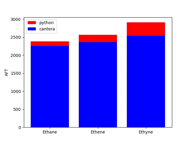

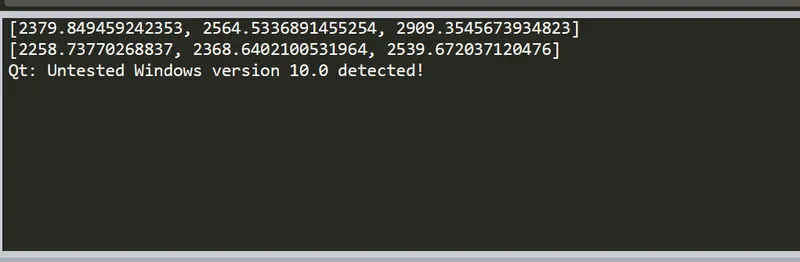
Adibatic flame temperature is highest fo Ethyne, followed by ethene and ethane respectively. Difference in values of AFT comapred between python code and cantera is fairly less for ethane but is more for ethene and ethyne.

4. Calculating Adiabatic flame temperature variation with respect to a number of Carbon atom chains.

`C_nH_(2n+2) + (3*n + 1)/2(O_2 + 3.76N_2) = nCO_2 + (n+1)H_2O + (3*n + 1)/2*3.76N_2`

"""
Adiabatic flame temperature variation with respect to a number of Carbon atom chains 
"""

# CnH2n+2 + (3*n + 1)/2(O2 + 3.76N2) = nCO2 + (n+1)H2O + (3*n + 1)/2*3.76N2 --- Stoichometric equation for Alkane

import matplotlib.pyplot as plt 

def h(T,coeffs):
 	R = 8.314 # J/mol*K

 	a1 = coeffs[0]
 	a2 = coeffs[1]
 	a3 = coeffs[2]
 	a4 = coeffs[3]
 	a5 = coeffs[4]
 	a6 = coeffs[5]

 	return (a1 + a2/2*T + a3/3*pow(T,2) + a4/4*pow(T,3) + a5/5*pow(T,4) + a6/T)*R*T
"""
 Defining coefficients of reactants
 """

o2_coeffs_r = [3.78245636E+00, -2.99673416E-03, 9.84730201E-06,  -9.68129509E-09, 3.24372837E-12, -1.06394356E+03, 3.65767573E+00]

n2_coeffs_r = [0.03298677E+02, 0.14082404E-02, -0.03963222E-04, 0.05641515E-07, -0.02444854E-10, -0.10208999E+04, 0.03950372E+02]

ch4_coeefs_r = [5.14987613E+00, -1.36709788E-02, 4.91800599E-05, -4.84743026E-08, 1.66693956E-11,-1.02466476E+04, -4.64130376E+00]

c2h6_coeffs_r = [4.29142492E+00, -5.50154270E-03, 5.99438288E-05, -7.08466285E-08, 2.68685771E-11, -1.15222055E+04, 2.66682316E+00]

c3h8_coeefs_r = [0.93355381E+00, 0.26424579E-01, 0.61059727E-05, -0.21977499E-07, 0.95149253E-11, -0.13958520E+05, 0.19201691E+02]

"""
Defining coefficients of product
"""

co2_coeffs_p = [3.85746029E+00, 4.41437026E-03, -2.21481404E-06, 5.23490188E-10, -4.72084164E-14, -4.87591660E+04, 2.27163806E+00]

h2o_coeffs_p = [3.03399249E+00, 2.17691804E-03, -1.64072518E-07, -9.70419870E-11, 1.68200992E-14, -3.00042971E+04, 4.96677010E+00]

n2_coeffs_p = [0.02926640E+02, 0.14879768E-02, -0.05684760E-05, 0.10097038E-09, -0.06753351E-13, -0.09227977E+04, 0.05980528E+02]


"""
Enthalpy of reactants
"""

T_std = 298.15

h_CH4_r = h(T_std,ch4_coeefs_r)
h_C2H6_r = h(T_std,c2h6_coeffs_r)
h_C3H8_r = h(T_std,c3h8_coeefs_r)
h_O2_r = h(T_std,o2_coeffs_r)
h_N2_r = h(T_std,n2_coeffs_r)

"""
Defining a function to calculate AFT
"""
def f(T):

	"""
	calculating enthalpy ofproducts
	"""

	h_CO2_p = h(T,co2_coeffs_p)
	h_H2O_p = h(T,h2o_coeffs_p)
	h_N2_p = h(T,n2_coeffs_p)

	if c == 1:

		h_reactants = h_CH4_r + ((3*c)+1/2*h_O2_r) + ((3*c)+1)/2*3.76*h_N2_r

		h_products = c*h_CO2_p + (c+1)*h_H2O_p + ((3*c)+1)/2*3.76*h_N2_p

	elif c == 2:

		h_reactants = h_C2H6_r + ((3*c)+1/2*h_O2_r) + ((3*c)+1)/2*3.76*h_N2_r

		h_products = c*h_CO2_p + (c+1)*h_H2O_p + ((3*c)+1)/2*3.76*h_N2_p

	else:

		h_reactants = h_C3H8_r + ((3*c)+1/2*h_O2_r) + ((3*c)+1)/2*3.76*h_N2_r

		h_products = c*h_CO2_p + (c+1)*h_H2O_p + ((3*c)+1)/2*3.76*h_N2_p

	return (h_products - h_reactants)


"""
Defining fprime
"""

def fprime(T):
	return (f(T+1e-6) - f(T))/(1e-6)

tol = 1e-4
T_aft = 3000
alpha = 0.2

"""
Defining a matrix for AFT values
"""
AFT_value = []

"""
Defining a matrix for no. of Carbon atoms
"""
Number_of_C_atom = []



for i in range (1,4):

	c = i

	Number_of_C_atom.append(c)

	while(abs(f(T_aft)) > tol):

		T_aft = T_aft - (alpha*f(T_aft)/fprime(T_aft))
	
	AFT_value.append(T_aft)

"""
Using Cantera to verify
"""


import cantera as ct 

gas = ct.Solution('gri30.xml')

"""
MAtrix for No. of carbon atoms
"""
Number_of_carbon_atoms = []

"""
Matrix for AFT values
"""
AFT_cantera = []

for i in range(1,4):

	c = i/1

	Number_of_carbon_atoms.append(c)

	if c == 1:

		gas.TPX = 298.15,101325,{'CH4':1, 'O2':((3*c)+1)/2, 'N2':((3*c)+1)/2*3.76}

		gas.equilibrate('HP','auto')

		AFT_cantera.append(gas.T)

	elif c == 2:

		gas.TPX = 298.15,101325,{'C2H6':1, 'O2':((3*c)+1)/2, 'N2':((3*c)+1)/2*3.76}

		gas.equilibrate('HP','auto')

		AFT_cantera.append(gas.T)

	else:

		gas.TPX = 298.15,101325,{'C3H8':1, 'O2':((3*c)+1)/2, 'N2':((3*c)+1)/2*3.76}

		gas.equilibrate('HP','auto')

		AFT_cantera.append(gas.T)




print(AFT_value)
print(AFT_cantera)
print(Number_of_C_atom)
print(Number_of_carbon_atoms)
plt.plot(Number_of_C_atom,AFT_value,color='red',label='python')
plt.plot(Number_of_carbon_atoms,AFT_cantera,color='blue',label='cantera')
plt.xlabel('Number of Carbon Atoms')
plt.ylabel('AFT')
plt.legend()
plt.show()

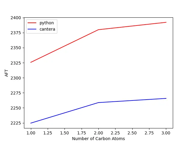
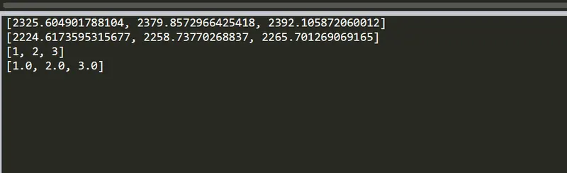
The plot of AFT values is similar for both the cases but the values are higher when calculated using cantera as it considers more number of species on the product side. The AFT increases withincrease in number of Carbon atoms.

• Conclusion :

1. Adibatic flame temperature calculation for different species can be done using python.
2. Cantera helps in calculating accurate value of AFT.
3. Cantera also helps in reducing time required for calculation as the code is fairly small.
4. Including more species on the product side will help us calculate AFT more accurately.
5. AFT values calculated using python are closer to actual values.