Week 3 - Adiabatic Flame Temperature calculation

OBJECTIVES :- To study an Adiabatic flame temperature by using two methods as-

1) Effect of equivalence ratio on AFT

2) Constant pressure reactor with heat loss

PROBLEM STATEMENTS :-

1) Effect of equivalence ratio on AFT-

Assume that methane is contained in a constant volume chamber. Write a program in python to plot the effect of equivalence ratio on the final adiabatic flame temperature. Compare the results with cantera. Assume that N2 is present.

Upload the results as a picture and python program.

We need to paste an image in our answer box and explain the results.

NOTE :- The correct trend for the AFT vs equivalence ratio will only be obtainable if we use the cantera module.

2) Constant pressure reactor with heat loss :-

1. Consider a constant pressure reactor with heat loss. The reactor is initially set at STP conditions.

2. The heat loss should be an input in our program and must be a fraction of the “maximum possible heat loss”. We should control heat loss using a variable called H_loss. e.g. H_loss = 0.5 would mean a heat loss that is equal to 50% of the maximum possible heat loss.

3. The fuel type can be a general hydrocarbon of the form CxHy. Phi and lambda = 1.0. Find the AFT of CH4 with H_loss = 0.35.

4. Test it only for -ane, -ene, -yne varients of 2 carbon atom chain and plot a trend. The provided therm.dat might not contain data for other alkanes, alkenes and alkynes.(in that case use cantera).

5. For a general alkane, plot the effect of the number of carbon atoms (from 1 to 3) on the final temperature. Assume H_loss = 0.

NOTE :- For comparisons between different species we are permitted to use Cantera.

INTRODUCTION & THEORY :-

To summarize, the adiabatic flame temperature for a given fuel oxidizer combination is determined by finding the final state temperature (i.e. the adiabatic flame temperature) for which the sum of the enthalpies of the reactants equal the sum of the enthalpies of the products.

For a combustion process that takes place adiabatically with no shaft work, the temperature of the products is reffered to as the adiabatic flame temperature. This is the maximum temperature that can be achieved for given reactants. Heat transfer, incomplete combustion and dissociation all results in lower temperature. The maximum adiabatic flame temperature for a given fuel and oxidizer combination occurs with a stoichiometric mixture (correct proportion such that all fuel and all oxidizer are consumed). The amount of excess air can be tailored as part of the design to control the adiabatic flame temperature.

We find the Adiabatic Flame Temperature in two ways-

• an approximate solution using an average value of Cp.

• A more accurate one using the tabulated evaluation of Cp with temperature.

IMPORTANCE IN PRACTICAL APPLICATIONS :-

In given combustion process, that takes place adiabatically and with no work or changes in kinetic or potential energy involved, the temperature of the products is reffered to as the “Adibatic flame temperature”.

1. It is used to charecterize the quality of fuel

2. It is used to determine suitability of fuel for an application.

3. It is used determined extent of substitution of a lower quality fuel to converse higher quality fuel

4. The adiabatic flame temperature is very important in design and scale up procedures wherever heat transfer is a significant considerations.

CODING APPROACH :-

Logic behind the code:- In this coding we define two adiabatic flame temperature- One for constant pressure combustion and other for constant volume. If a fuel air mixture burns adiabatically at constant pressure, the absolute enthalpy of the reactants at the initial state (i.e. T = 298.15K, P = 1atm) equals the absolute enthalpy of the products at the final state (T = Tad, P = 1atm)-

Hreact(Ti, P) = Hprod(Tad, P)

or equivalently, on a per mass of mixture basis,

hreact(Ti, P) = hprod(Tad, P).

This first low statement defines what is called the constant pressure adiabatic flame temperature.

Step wise procedures :-

Combine process of all the python files are as below-

1. First off all importing some important modules like matplotlib, numpy and cantera.

2. Define the function of temperature and coefficients

3. Define known values of universal gas constants

4. Define all arrays which we need to describe polynomial equations

5. return the polynomial equation

6. Defining the coefficients of the elements taken from NASA thermodynamic data file.

Seperate coding steps for each file are as follows-

(A) CODE-1 :-

1. Define the function of temperature and psi (i.e. coefficients of elements)

2. Define enthalpies of reactants

3. Define enthalpies of products

4. Apply the conditions such as, psi > 1 (for lean mixture) and psi < 1 (for reach mixture)

5. Return difference of enthalpies of products, reactants and number of products and rectants)

6. Consider guess temperature is 1500K and linspace command from 0.6 to 1.6 by difference of 0.1

7. Under relaxed factor depends on, after what much iterations we get the converged solution.

8. Use for loop in the range of zero to linspace.

9. Apply Newton Raphson formula and appended it in T_AFT.

10. It repeats upto the solution not converged belw tollerance.

11. For comparing this import cantera module.

12. Define any gas solutions

13. Calculate total mole and find out each mole fractions

14. TPX → Temperature, pressure and mole fraction

15. Calculate equivalence ratio.

16. Plot “Equivalence ratio vs T_AFT”.

import numpy as np
import matplotlib.pyplot as plt
#CH4 + 2(O2 + 3.76N2) = CO2 + 2H2O + 7.52N2
# Determining AFT using Newton Raphson Method
def h(T,Coeff):
	R = 8.314			#Universal gas constant

	#Arrays
	a1 = Coeff[0]
	a2 = Coeff[1]
	a3 = Coeff[2]
	a4 = Coeff[3]
	a5 = Coeff[4]
	a6 = Coeff[5]
	#Polynomial equation
	return (a1 + a2*T/2 + a3*pow(T,2)/3 + a4*pow(T,3)/4 + a5*pow(T,4)/5 + a6/T)*R*T

	#Defining the coefficients of the elements
CH4_coeffs_l = [5.14987613E+00,-1.36709788E-02,4.91800599E-05,-4.84743026E-08,1.66693956E-11,-1.02466476E+04,-4.64130376E+00]
O2_coeffs_l = [3.78245636E+00,-2.99673416E-03,9.84730201E-06,-9.68129509E-09,3.24372837E-12,-1.06394356E+03,3.65767573E+00]
N2_coeffs_l = [0.03298677E+02,0.14082404E-02,-0.03963222E-04,0.05641515E-07,-0.02444854E-10,-0.10208999E+04,0.03950372E+02]
N2_coeffs_h = [0.02926640E+02,0.14879768E-02,-0.05684760E-05,0.10097038E-09,-0.06753351E-13,-0.09227977E+04,0.05980528E+02]
CO2_coeffs_h = [3.85746029E+00,4.41437026E-03,-2.21481404E-06,5.23490188E-10,-4.72084164E-14,-4.87591660E+04,2.27163806E+00]
H2O_coeffs_h = [3.03399249E+00,2.17691804E-03,-1.64072518E-07,-9.70419870E-11,1.68200992E-14,-3.00042971E+04,4.96677010E+00]
O2_coeffs_h = [3.28253784E+00,1.48308754E-03,-7.57966669E-07,2.09470555E-10,-2.16717794E-14,-1.08845772E+03,5.45323129E+00]
CO_coeffs_h = [2.71518561E+00,2.06252743E-03,-9.98825771E-07,2.30053008E-10,-2.03647716E-14,-1.41518724E+04,7.81868772E+00]

def f(T,psi):
	Tstp = 298.15	#K
	R = 8.314 		#J/mol-K

	#Enthaplies of reactants
	h_CH4_r = h(Tstp, CH4_coeffs_l)
	h_O2_r = h(Tstp, O2_coeffs_l)
	h_N2_r = h(Tstp, N2_coeffs_l)

	#Enthalpies of products
	h_CO2_p = h(T, CO2_coeffs_h)
	h_H2O_p = h(T, H2O_coeffs_h)
	h_O2_p = h(T, O2_coeffs_h)
	h_N2_p = h(T, N2_coeffs_h)
	h_CO_p = h(T, CO_coeffs_h)

	#Applying conditions
	if psi > 1: 	#Lean mixture
		h_reactants = h_CH4_r + 2*psi*h_O2_r + 7.52*psi*h_N2_r
		h_products = h_CO2_p + 2*h_H2O_p + (2*psi-2)*h_O2_p + 7.52*psi*h_N2_p
		N_reactants = 1 + 2*psi + 7.52*psi
		N_products = 1 + 2 + (2*psi - 2) + 7.52*psi

	else:		#Rich mixture
		h_reactants = h_CH4_r + 2*psi*h_O2_r + 7.52*psi*h_N2_r
		h_products = (4*psi - 3)*h_CO2_p + 2*h_H2O_p + (4-4*psi)*h_CO_p + 7.52*psi*h_N2_p
		N_reactants = 1 + 2*psi + 7.52*psi
		N_products = (4*psi - 3) + 2 + (4-4*psi) + 7.52*psi

	return h_products - h_reactants -R*(N_products*T - N_reactants*Tstp)

def fprime(T, psi):
	return (f(T + 1e-6, psi) - f(T,psi))/1e-6

T_guess = 1500
tol = 1e-3 
iter = 0
alpha = 0.2 	#Under relaxed factor

psi = np.linspace(0.6, 1.6, 11)

T_AFT = []

for i in range (0, len(psi)):
	while (abs(f(T_guess, psi[i])) > tol):
		#Newton Raphson method
		T_guess = T_guess - alpha*((f(T_guess,psi[i])/fprime(T_guess, psi[i])))
		iter = iter + 1
	T_AFT.append(T_guess)


# Determining AFT using cantera
import cantera as ct
gas = ct.Solution("gri30.xml")

T_AFT_cantera = []

for i in range (0, len(psi)):
	#Mole fraction values
	Total_mole = 1 + 2*psi[i] + 7.52*psi[i]
	mole_fraction_CH4 = 1/Total_mole
	mole_fraction_O2 = (2*psi[i])/Total_mole
	mole_fraction_N2 = (7.52*psi[i])/Total_mole

	#TPX -> Temperature, pressure, mole fraction
	gas.TPX = 298.15, 101325, {"CH4": mole_fraction_CH4, "O2": mole_fraction_O2, "N2": mole_fraction_N2}
	gas.equilibrate("UV", "auto")
	T_AFT_cantera.append(gas.T)

Equivalence_ratio = 1/psi

#Figures
plt.plot(Equivalence_ratio, T_AFT, color = "blue")
plt.plot(Equivalence_ratio, T_AFT_cantera, color = "red")
plt.xlabel("Equivalence_ratio")
plt.ylabel("Adiabatic Flame Temperature(K)")
plt.grid("on")		# or plt.grid()
plt.title("Effect of Equivalence ratio on the AFT")
plt.legend(["Python","Cantera"])
plt.savefig("Effect of Equivalence ratio on the AFT")
plt.show()

RESULTS-1 :-

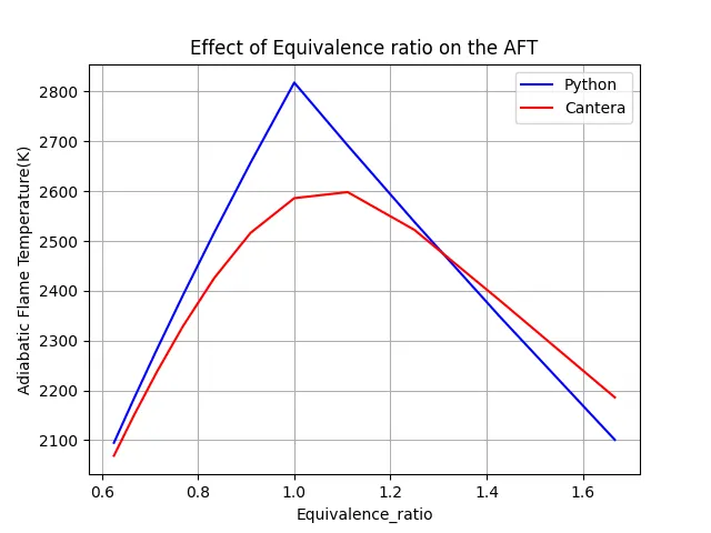
Here, red colour curve for cantera plot and blue colour curve for python plots. Python curve shows maximum temperature i.e. > 2800K and cantera curve shows maximum temperature = 2600K. Python gives conical shape plot whereas cantera gives parabolic shape plots. Cantera values within python values. X-axis shows Equivalence ratio and Y-axis shows Adiabatic flame temperature. Both the plots showining same range on X-axis i.e. Equivalence ratio.

(B) CODE-2 :-

In this program not need to find out type of fuel mixtures.

First calculate difference in enthalpy of product and reactants and addition of heat loss. Use the Newton Raphson method and plot the graph as shown below.

#In this program we are going to calculate the AFT of methane at different equivalence ratios
#CH4 + 2(O2 + 3.76N2) = CO2 + 2H2O + 7.52N2
import matplotlib.pyplot as plt
import numpy as np
import math
def h(T, co_effs):
	#Function to evaluate enthalpy
	R = 8.314   #J/mole-k		#Universal gas constant

	#Arrays
	a1 = co_effs[0]
	a2 = co_effs[1]
	a3 = co_effs[2]
	a4 = co_effs[3]
	a5 = co_effs[4]
	a6 = co_effs[5]

	#Polynomial equations
	return (a1 + a2*T/2 + a3*pow(T,2)/3 + a4*pow(T,3)/4 + a5*pow(T,4)/5 + a6/T)*R*T

#Defining the co-efficients of elements
CH4_coeffs_l = [5.14987613E+00,-1.36709788E-02,4.91800599E-05,-4.84743026E-08,1.66693956E-11,-1.02466476E+04,-4.64130376E+00]
O2_coeffs_l = [3.78245636E+00,-2.99673416E-03,9.84730201E-06,-9.68129509E-09,3.24372837E-12,-1.06394356E+03,3.65767573E+00]
N2_coeffs_l = [0.03298677E+02,0.14082404E-02,-0.03963222E-04,0.05641515E-07,-0.02444854E-10,-0.10208999E+04,0.03950372E+02]
N2_coeffs_h = [0.02926640E+02,0.14879768E-02,-0.05684760E-05,0.10097038E-09,-0.06753351E-13,-0.09227977E+04,0.05980528E+02]
CO2_coeffs_h = [3.85746029E+00,4.41437026E-03,-2.21481404E-06,5.23490188E-10,-4.72084164E-14,-4.87591660E+04,2.27163806E+00]
H2O_coeffs_h = [3.03399249E+00,2.17691804E-03,-1.64072518E-07,-9.70419870E-11,1.68200992E-14,-3.00042971E+04,4.96677010E+00]

Heat_loss = 0.35

def f(T):
	#Function represents root finding problem
	Tstp = 298.15
	LHV = 800950

	#Enthalpies of the product
	h_CO2_p = h(T, CO2_coeffs_h)
	h_N2_p = h(T, N2_coeffs_h)
	h_H2O_p = h(T, H2O_coeffs_h)

	H_products = h_CO2_p + 2*h_H2O_p + 7.52*h_N2_p
	print(H_products)

	#Enthalpies of the reactants
	Tstp = 298.15
	h_CH4_r = h(Tstp, CH4_coeffs_l)
	h_O2_r = h(Tstp, O2_coeffs_l)
	h_N2_r = h(Tstp, N2_coeffs_l)

	H_reactants = h_CH4_r + 2*h_O2_r + 7.52*h_N2_r
	print(H_reactants)
	Loss = Heat_loss*LHV

	return H_products - H_reactants + Loss


def fprime(T):
	return (f(T + 1e-6) - f(T))/1e-6

T_guess = 1500
tol = 1e-3 
iter = 0
alpha = 0.2
while(abs(f(T_guess)) > tol):
	#Newton Raphson method
	T_guess = T_guess - alpha*((f(T_guess))/(fprime(T_guess)))
	iter = iter + 1
	plt.plot(iter, T_guess, "*", color = "gold")

print(T_guess)
plt.xlabel("Number of Iterations")
plt.ylabel("Adiabatic flame temperature for 0.35 heat loss")
print(iter)
plt.savefig("No of iterations vs AFT")
plt.show()

RESULTS-2 :-

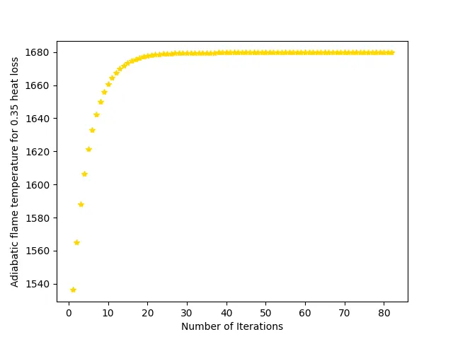
This plot has Number of iterations vs Adiabatic flame temperature. This plot totally depends on the under relaxed values i.e. alpha. Upto 10 to 15 number of iterations adiabatic flame temperature increases fastly and then it remain constant over number of iterations. The maximum adiabatic flame temperature is 1680K.

(C) CODE-3 :-

In this program we have three elements i.e. alkanes, alkenes and alkynes. Reaction for each elements is somewhat different. The detail steps as below-

1. Define the function for alkanes

2. Define standerd temperature, heat loss and LHV (i.e. low heat value), enthalpies of reactants and products and return it is prime value.

3. Same way define for alkene and alkynes as shown in code.

4. The only key difference is that multiplication of coefficient of Nitrogen i.e. in alkane it is 3.5, in alkene it is 3 and in alkynes it is 2.5, as shown in code.

5. Use the Newton Raphson method formula and finally plot the graph “iterations vs T_guess”.

import matplotlib.pyplot as plt
import numpy as np 
import cantera as ct 
 
def h(T, Coeff):
	R = 8.314	#j/mole-K 		#Universal gas constant

	#Arrays
	a1 = Coeff[0]
	a2 = Coeff[1]
	a3 = Coeff[2]
	a4 = Coeff[3]
	a5 = Coeff[4]
	a6 = Coeff[5]
	
	#Polynomial equation
	return (a1 + a2*T/2 + a3*pow(T,2)/3 + a4*pow(T,3)/4 + a5*pow(T,4)/5 + a6/T)*R*T

# Defining the coefficients of the elements taken from NASA thermodynamic data
C2H6_coeff_l = [4.29142492E+00,-5.50154270E-03,5.99438288E-05,-7.08466285E-08,2.68685771E-11,-1.15222055E+04,2.66682316E+00]
C2H4_coeff_l = [3.95920148E+00,-7.57052247E-03,5.70990292E-05,-6.91588753E-08,2.69884373E-11,5.08977593E+03,4.09733096E+00]
C2H2_coeff_l = [8.08681094E-01,2.33615629E-02,-3.55171815E-05,2.80152437E-08,-8.50072974E-12,2.64289807E+04,1.39397051E+01]
O2_coeffs_l = [3.78245636E+00,-2.99673416E-03,9.84730201E-06,-9.68129509E-09,3.24372837E-12,-1.06394356E+03,3.65767573E+00]
N2_coeffs_l = [0.03298677E+02,0.14082404E-02,-0.03963222E-04,0.05641515E-07,-0.02444854E-10,-0.10208999E+04,0.03950372E+02]
N2_coeffs_h = [0.02926640E+02,0.14879768E-02,-0.05684760E-05,0.10097038E-09,-0.06753351E-13,-0.09227977E+04,0.05980528E+02]
CO2_coeffs_h = [3.85746029E+00,4.41437026E-03,-2.21481404E-06,5.23490188E-10,-4.72084164E-14,-4.87591660E+04,2.27163806E+00]
H2O_coeffs_h = [3.03399249E+00,2.17691804E-03,-1.64072518E-07,-9.70419870E-11,1.68200992E-14,-3.00042971E+04,4.96677010E+00]

def f_Alkane(T):
	#C2H6 + 3.5*3.76N2 = 2CO2 + 3.5*3.76N2 + 0.35*LHV

	Tstp = 298.15	#K 			#Standerd temperature
	Heat_loss = 0.35
	LHV = 1428275	#J/mole 	#Low heat value

	#Enthalpies of reactants
	h_C2H6_r = h(Tstp,C2H6_coeff_l)
	h_O2_r = h(Tstp, O2_coeffs_l)
	h_N2_r = h(Tstp, N2_coeffs_l)

	#Enthalpies of products
	h_N2_p = h(T,N2_coeffs_h)
	h_CO2_p = h(T,CO2_coeffs_h)
	h_H2O_p = h(T, H2O_coeffs_h)

	h_reactants = h_C2H6_r + 3.5*h_O2_r + (3.5*3.76*h_N2_r)
	h_products = 2*h_CO2_p + 3*h_H2O_p + (3.5*3.76*h_N2_p)

	Loss = Heat_loss*LHV
	return h_products - h_reactants + Loss

def fprime_Alkane(T):
	return (f_Alkane(T+1e-6) - f_Alkane(T))/1e-6

def f_Alkene(T):
	#C2H4 + 3O2 + 3*3.76N2 = 2CO2 + 2H2O + 3*3.76N2 + 0.35*LHV

	Tstp = 298.15		#Standerd temperature
	Heat_loss = 0.35
	LHV = 1323474		#Low heat value

	#Enthalpies of reactants
	h_C2H4_r = h(Tstp, C2H4_coeff_l)
	h_O2_r = h(Tstp, O2_coeffs_l)
	h_N2_r = h(Tstp, N2_coeffs_l)

	#Enthalpies of products
	h_N2_p = h(T, N2_coeffs_h)
	h_CO2_p = h(T, CO2_coeffs_h)
	h_H2O_p = h(T, H2O_coeffs_h)

	h_reactants = h_C2H4_r + 3*h_O2_r + (3*3.76*h_N2_r)
	h_products = 2*h_CO2_p + 2*h_H2O_p + (3*3.76*h_N2_p)

	Loss = Heat_loss*LHV

	return h_products - h_reactants + Loss

def fprime_Alkene(T):
	return (f_Alkene(T + 1e-6) - f_Alkene(T))/1e-6

def f_Alkyne(T):
	#C2H2 + 2.5O2 + 2.5*3.76N2 = 2CO2 + H2O + 3.5*3.76N2 + 0.35*LHV

	Tstp = 298.15 		#Standerd temperature
	Heat_loss = 0.35
	LHV = 1258020		#Low heat value

	#Enthalpies of reactants
	h_C2H2_r = h(Tstp, C2H2_coeff_l)
	h_O2_r = h(Tstp, O2_coeffs_l)
	h_N2_r = h(Tstp, N2_coeffs_l)

	#Enthalpies of products
	h_N2_p = h(T, N2_coeffs_h)
	h_CO2_p = h(T, CO2_coeffs_h)
	h_H2O_p = h(T, H2O_coeffs_h)

	h_reactants = h_C2H2_r + 2.5*h_O2_r + (2.5*3.76*h_N2_r)
	h_products = 2*h_CO2_p + h_H2O_p + (3.5*3.76*h_N2_p)

	Loss = Heat_loss*LHV

	return h_products - h_reactants + Loss

def fprime_Alkyne(T):
	return (f_Alkyne(T+1e-6) - f_Alkyne(T))/1e-6


T_Alkane = 1500
T_Alkene = 1500
T_Alkyne = 1500
tol = 1e-3 
alpha = 1
T_AFT = []

#By using Newton Raphson method
while (abs(f_Alkane(T_Alkane)) > tol):
	T_Alkane = T_Alkane - alpha*(f_Alkane(T_Alkane)/fprime_Alkane(T_Alkane))
T_AFT.append(T_Alkane)

while (abs(f_Alkene(T_Alkene)) > tol):
	T_Alkene = T_Alkene - alpha*(f_Alkene(T_Alkene)/fprime_Alkene(T_Alkene))
T_AFT.append(T_Alkene)

while (abs(f_Alkyne(T_Alkyne)) > tol):
	T_Alkyne = T_Alkyne - alpha*(f_Alkyne(T_Alkyne)/fprime_Alkyne(T_Alkyne))
T_AFT.append(T_Alkyne)

#Available fuels
fuel = ["Ethane", "Ethene", "Ethyne"]
print(T_AFT)

#Figures
plt.bar(fuel, T_AFT)
plt.xlabel("Type of Hydrocarbon")
plt.ylabel("Flame Temperature(K)")
plt.title("Estimation of FT for a heat loss factor of 0.35")
plt.savefig("Types of Hydrocarbon vs Flame Temperature")
plt.show()

RESULTS-3 :-

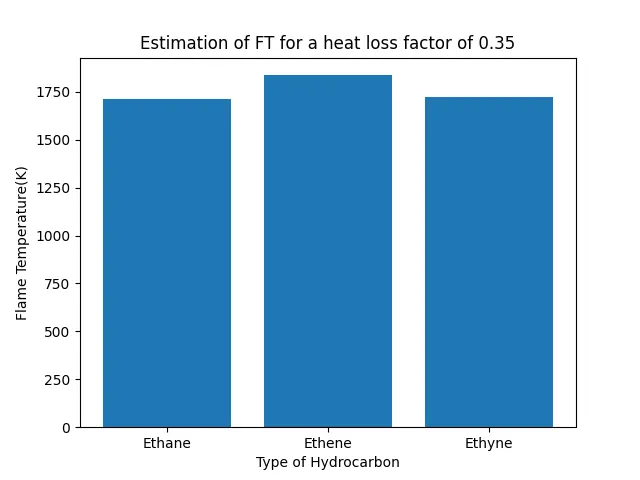
This plot shows flame temperature vs types of hydrocarbon. In this plot I find out flame temperature at 0.35 heat loss factor. From this plot we can conclude that flame temperature for ethane and ethyne is same which is smaller than Ethene. From this bar graph we can conclude that flame temperature for alkene i.e. ethene is maximum. At same factor of heat loss we get different result for ethane, ethene and ethyne.

Temperature for Ethane and Ethyne = 1714K

Temperature for Ethene = 1837K

Temperature of Ethyne = 1722K.

CONCLUSIONS :-

From above codes and plots we can conclude following points are-

1. Cantera gives more better results than python plot in chemical compositions.

2. In python code more temperature release than cantera code also the code script is lesser in cantera as compare to python script.

3. According to reaction we need to define enthalpies for reactant and products side.

4. Newton Raphson method is depends on under relaxed factor i.e. alpha.

5. Flame temperature is nearly same for alkane and alkynes while flame temperature is higher for alkene, it shown in bar plot.

6. We can find the types of mixture i.e. lean or rich or stoichometric from psi value i.e. fuel to air ratio.

7. Psi = Fuel quantity/Air quantity.

In this way, I completed this challenge by applying all given conditions. Write the code in python and cantera also plot the respective graph, find the flame temperature for Alkane, Alkene and Alkynes and finally I write the Conclussion on them.