Week 3.5 - Deriving 4th order approximation of a 2nd order derivative using Taylor Table method
AIM :
To derive the following 4th order approximations of the second-order derivative by using Taylor's table method, analytical function exp(x)*cos(x) and compare the result with three different numerical approximations.
Finite-Difference Methods
In numerical analysis, finite-difference methods (FDM) are a class of numerical techniques for solving differential equations by approximating derivatives with finite differences.
1. Central difference : Central differences are useful in solving partial differential equations.
2. Skewed right-sided difference : A right-skewed distribution has a long right tail. Right-skewed distributions are also called positive-skew distributions.
3. Skewed left-sided difference :A left-skewed distribution has a long left tail. Left-skewed distributions are also called negatively-skewed distributions.
The equations used for 4th order approximations of the second-order derivative was derived from p+q, where 'p' stands for order of derivative and 'q' stands for order of approximation.
1. Central difference = (p+q-1) = (2+4-1) = 5
2. Skewed right-sided difference = (p+q) = (2+4) = 6
3. Skewed left-sided difference = (p+q) = (2+4) = 6
PROCEDURE :
FORMULATION FOR THE TAYLOR SERIES METHOD FOR CENTRAL DIFFERENCE METHOD :
f"(x) = `(af(x-2h) + bf(x-h) +cf(x)+df(x+h)+ef(x+2h)) / (Delta(x^2))`
FORMULATION FOR THE TAYLOR SERIES METHOD FOR LEFT SKEWED DIFFERENCE METHOD :
`(af(x) + bf(x-h) +cf(x-2h)+df(x-3h)+ef(x-4h)+gf(x-5h)) / (Delta(x^2))`
FORMULATION FOR THE TAYLOR SERIES METHOD FOR RIGHT SKEWED DIFFERENCE METHOD :
`(af(x) + bf(x+h) +cf(x+2h)+df(x+3h)+ef(x+4h)+gf(x+5h)) / (Delta(x^2))`
Now, lets take second-order derivative for 4th order approximations for
TAYLORS TABLE FOR CENTRAL DIFFERENCE METHOD :
`(del^2f)/(delx^2) = af_(i-2)+bf_(i-1)+cf_(i)+df_(i+1)+ef(i+2)`
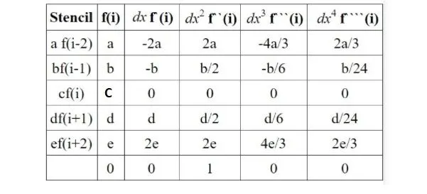
MATLAB CODE TO FIND THE ABOVE COEFFICIENTS :
clear all
close all
clc
% find coefficient
A = [1 1 1 1 1;-2 -1 0 1 2;2 1/2 0 1/2 2;-4/3 -1/6 0,1/6 4/3;2/3 1/24 0 1/24 2/3];
B = [0;0;1;0;0];
C = inv(A)*B;
RESULT :
C =
a = -0.0833b = 1.3333
c = -2.5000
d = 1.3333
f = -0.0833
Now, we have to calculate the error i.e difference between the Central difference and analytical derivative
TAYLORS TABLE FOR RIGHT SKEWED DIFFERENCE METHOD :
`(del^2f)/(delx^2) = af_(i)+bf_(i+1)+cf(i+2)+df(i+3)+ef(i+4)+gf(i+5)`
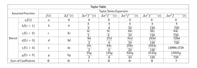
MATLAB CODE TO FIND THE ABOVE COEFFICIENTS :
clear all
close all
clc
% find coefficient
A = [1 1 1 1 1 1;0 1 2 3 4 5;0 1/2 2 9/2 8 25/2;0 1/6 8/6 27/6 64/6 125/6;0 1/24 16/24 81/24 256/24 625/24;0 1/120 32/120 243/120 1024/120 3125/120];
B =[0;0;1;0;0;0];
C=A\B;
C =
3.7500
-12.8333
17.8333
-13.000
5.0833
-0.8333
TAYLORS TABLE FOR LEFT SKEWED DIFFERENCE METHOD :
`(del^2f)/(delx^2) = af_(i)+bf_(i-1)+cf(i-2)+df(i-3)+ef(i-4)+gf(i-5)`
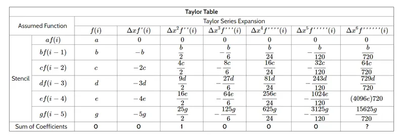
MATLAB CODE TO FIND THE ABOVE COEFFICIENTS :
clear all
close all
clc
% find coefficient
A = [1 1 1 1 1 1;0 -1 -2 -3 -4 -5;0 1/2 2 9/2 8 25/2;0 -1/6 -8/6 -27/6 -64/6 -125/6;0 1/24 16/24 81/24 256/24 625/24;0 -1/120 -32/120 -243/120 -1024/120 -3125/120];
B =[0;0;1;0;0;0];
c=inv(A)*B
RESULT :
C =
3.7500
-12.8333
17.8333
-13.000
5.0833
-0.8333
MAIN CODE :
clear all
close all
clc
% input values
x = pi/3;
dx = linspace(pi/4000,pi/40,20);
%second order analytical function = exp(x)*cos(x)
% analytical_derivative
second_order_analytical_derivative = -2*sin(x)*exp(x);
% for loop function
for i = 1:length(dx)
central_difference_error(i) = central_difference(x,dx(i));
skewed_right_error(i) = skewed_right_side(x,dx(i));
skewed_left_error(i) = skewed_left_side(x,dx(i));
end
RESULT :
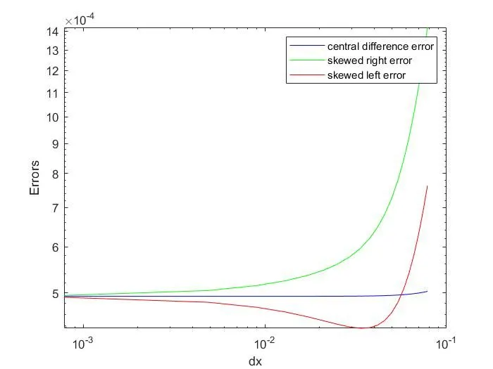
The comparsion of the above graph shows the absolute error between the central_difference_error,skewed_right_error,
skewed_left_error.
The central scheme is more aacurate than the skewed differencing.
Comparing the other errors, the skewed right error is high as the dx value increases. The skewed scheme is used when
we predict using the boundary condition at one direction or points, where central scheme requires information both direction
of the point.