Week 3.5 - Deriving 4th order approximation of a 2nd order derivative using Taylor Table method

To derive the 4th order approximation schemes, the taylor table method is used.

i) Central Difference Scheme

For the 4th order approximation of the 2nd order derivative using the central difference scheme the stencil contains 5 nodes in it. The following table represents taylor table representation of it

	`f_i`	`trianglex f_i^1`	`trianglex^2 f_i^2`	`trianglex^3 f_i^3`	`trianglex^4 f_i^4`	`trianglex^5 f_i^5`
`a f_(i-2)`	a	-2 a	2 a	-4/3 a	2/3 a	-4/15 a
`b f_(i-1)`	b	-b	1/2 b	-1/6 b	1/24 b	-1/32 b
`c f_i`	c
`d f_(i+1)`	d	d	1/2 b	1/6 d	1/24 d	1/32 d
`e f_(i+2)`	e	2 e	2e	-4/3 e	2/3 e	4/15 e

On solving this system of equations on MATLAB using the following code, we get the final result as

clear all
close all
clc

%Declaring the oeficient matrix
A= [1 -2 2 -4/3 2/3; 1 -1 1/2 -1/6 1/24;1 0 0 0 0;1 1 1/2 1/6 1/24;1 2 2 4/3 2/3];
%Declaring the RHS
B= [0 ;0 ;1 ;0 ;0];
%solving for X in AX=B
X=linsolve(A',B);

`(d^2 f )/dx^2 = (-f_(i-2) + 16 f_(i-1) -30 f_i +16 f_(i+1) - f_(i+2)) /(12 trianglex^2)`

On substituting the values of a through e in the equation for coefficient for the fifth derivative, we get zero. Therefore, the leading order error term is the 6th derivative, and since the order of the 6th derivative is 4, the order of the derived approximation is 4.

ii)Skewed right sided Scheme

For the 4th order approximation of the 2nd order derivative using the Forward difference scheme, the stencil contains 6 nodes in it. The following table represents taylor table representation of it

	`f_i`	`trianglex f_i^1`	`(trianglex^2)/2 f_i^2`	`(trianglex^3)/6 f_i^3`	`(trianglex^4)/24 f_i^4`	`(trianglex^5)/120 f_i^5`	`(trianglex^6)/720 f_i^6`
`a f_i`	a
`b f_(i+1)`	b	b	b	b	b	b	b
`c f_(i+2)`	c	2 c	4 c	8 c	16 c	32 c	64 c
`d f_(i+3)`	d	3 d	27 d	81 d	243 d	729 d	2187 d
`e f_(i+4)`	e	4 e	16 e	64 e	256 e	1024 e	4096 e
`f f_(i+5)`	f	5 f	25 f	125 f	625 f	3125 f	15625 f

On solving this system of equations on MATLAB using the following code, we get the final result as

clear all
close all
clc

%Declaring the oeficient matrix
A= [1 0 0 0 0 0; 
    1 1 1/factorial(2) 1/factorial(3) 1/factorial(4) 1/factorial(5); 
    1 2 (2^2)/factorial(2) (2^3)/factorial(3) (2^4)/factorial(4) (2^5)/factorial(5); 
    1 3 (3^2)/factorial(2) (3^3)/factorial(3) (3^4)/factorial(4) (3^5)/factorial(5);
    1 4 (4^2)/factorial(2) (4^3)/factorial(3) (4^4)/factorial(4) (4^5)/factorial(5);
    1 5 (5^2)/factorial(2) (5^3)/factorial(3) (5^4)/factorial(4) (5^5)/factorial(5);];

%Declaring the RHS
B= [0 ;0 ;1 ;0 ;0 ;0];

%solving for X in AX=B
X=linsolve(A',B);

%Evaluating the coefficient of the 6th derivative
D = 1/factorial(6) * [0 1 2^6 3^6 4^6 5^6] * X;

`(d^2 f )/dx^2 = (45f_(i) - 154 f_(i+1) + 214 f_(i+2) -156 f_(i+3) + 61 f_(i+4) - 10 f_(i+5)) /(12 trianglex^2)`

On substituting the values of a through f in the equation for coefficient for the sixth derivative, we get a non zero value. Therefore, the leading order error term is the 6th derivative, and since the order of the 6th derivative is 4, the order of the derived approximation is 4.

iii) Skewed Left side

For the 4th order approximation of the 2nd order derivative using the Backward difference scheme, the stencil contains 6 nodes in it. The following table represents taylor table representation of it

	`f_i`	`trianglex f_i^1`	`(trianglex^2)/2 f_i^2`	`(trianglex^3)/6 f_i^3`	`(trianglex^4)/24 f_i^4`	`(trianglex^5)/120 f_i^5`	`(trianglex^6)/720 f_i^6`
`a f_i`	a
`b f_(i-1)`	b	-b	b	-b	b	-b	b
`c f_(i-2)`	c	-2 c	4 c	-8 c	16 c	-32 c	64 c
`d f_(i-3)`	d	-3 d	27 d	-81 d	243 d	-729 d	2187 d
`e f_(i-4)`	e	-4 e	16 e	-64 e	256 e	-1024 e	4096 e
`f f_(i-5)`	f	-5 f	25 f	-125 f	625 f	-3125 f	15625 f

On solving this system of equations on MATLAB using the following code, we get the final result as

clear all
close all
clc

%Declaring the oeficient matrix
A= [1 0 0 0 0 0; 
    1 1 1/factorial(2) 1/factorial(3) 1/factorial(4) 1/factorial(5); 
    1 2 (2^2)/factorial(2) (2^3)/factorial(3) (2^4)/factorial(4) (2^5)/factorial(5); 
    1 3 (3^2)/factorial(2) (3^3)/factorial(3) (3^4)/factorial(4) (3^5)/factorial(5);
    1 4 (4^2)/factorial(2) (4^3)/factorial(3) (4^4)/factorial(4) (4^5)/factorial(5);
    1 5 (5^2)/factorial(2) (5^3)/factorial(3) (5^4)/factorial(4) (5^5)/factorial(5);];

%Declaring the RHS
B= [0 ;0 ;1 ;0 ;0 ;0];

%solving for X in AX=B
X=linsolve(A',B);

%Evaluating the coefficient of the 6th derivative
D = 1/factorial(6) * [0 1 2^6 3^6 4^6 5^6] * X;

`(d^2 f )/dx^2 = (45f_(i) - 154 f_(i+1) + 214 f_(i+2) -156 f_(i+3) + 61 f_(i+4) - 10 f_(i+5)) /(12 trianglex^2)`

On substituting the values of a through f in the equation for coefficient for the sixth derivative, we get a non zero value. Therefore, the leading order error term is the 6th derivative, and since the order of the 6th derivative is 4, the order of the derived approximation is 4.

Moving on, the next step was to use the derived expressions to evaluate `f(x) = e^x cosx`

First, the analytical derivative is evaluated as follows,

`f'(x) = e^x (cosx - sin x)`

`f''(x) = - 2 e^x sinx` ;

For the current exercise, the derivatice is evaluated for x=pi/2. Four different step sizes, 0.0001,0.001,0.01, and 0.1 are used. The following code is used to evaluate the derivative through the 3 approximation schemes:

% Main code to solve, plot and create the animation file

clear all
close all
clc

% defining x, dx
x = pi/2;
dx = [0.0001,0.001,0.01,0.1];

%Analytical derivative
analytical = -2 * exp(x) * sin(x);

%initializing the error term arrays
error_cent = zeros;
error_fwd = zeros;
error_bwd = zeros;

%Looping over the range
for i=1:length(dx) 
    % Cent
    order_cent = ( - evaluator(x-2*dx(i)) + 16 * evaluator(x-dx(i)) - 30 * evaluator(x) + 16 * evaluator(x+dx(i))  - evaluator(x+2*dx(i)))/(12*dx(i)^2); 
    error_cent(i) = abs(order_cent-analytical);

    % Forward
    order_fwd = (45 *  evaluator(x) - 154 * evaluator(x+dx(i)) + 214 * evaluator(x+2*dx(i)) - 156 * evaluator(x+3*dx(i)) + 61 * evaluator(x+4*dx(i)) - 10 * evaluator(x+5*dx(i)))/ (12*dx(i)^2);
    error_fwd(i) = abs(order_fwd-analytical);

    % Backward
    order_bwd = (45 *  evaluator(x) - 154 * evaluator(x-dx(i)) + 214 * evaluator(x-2*dx(i)) - 156 * evaluator(x-3*dx(i)) + 61 * evaluator(x-4*dx(i)) - 10 * evaluator(x-5*dx(i)))/ (12*dx(i)^2);;  
    error_bwd(i) = abs(order_bwd-analytical);
end

%Plot
loglog(dx,error_cent,'r',dx,error_fwd,'b',dx,error_bwd,'g')
xlabel('STEP SIZE')
ylabel('ERROR')


% Function to evaluate the function
function answer = evaluator(x)
   
    answer = exp (x) * cos (x);
    
end

On running the code the following plot is obtained

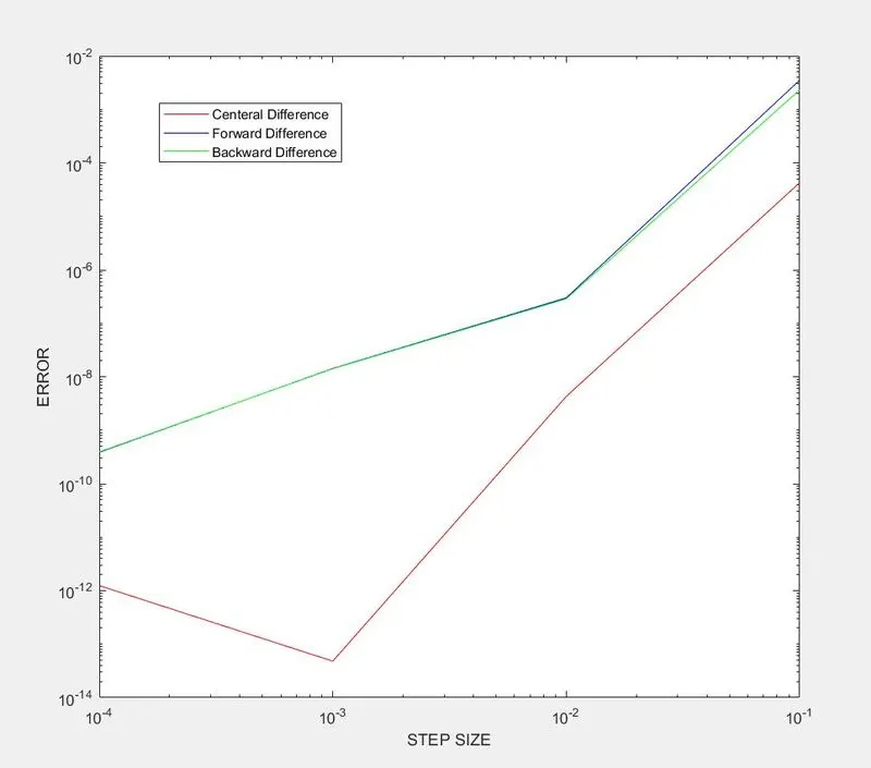
From the plot it can be seen that

1) The central difference scheme has the lowest error amongst the 3 schemes for all the step sizes. It can also be seen that the error is minimum for a step size of 0.001.

2) The backward difference scheme has a lower error than the forward difference scheme for large step sizes. With smaller step sizes, both forward and central provide similar errors.