Week 3.5 - Deriving 4th order approximation of a 2nd order derivative using Taylor Table method
Deriving 4th order approximation of a 2nd order derivative using Taylor Table method
Aim : Deriving 4th order approximation of a 2nd order derivative using Taylor Table method
Objective: To Deriving 4th order approximation of a 2nd order derivative using Taylor Table method for
1. Central difference
2. Skewed right-sided difference
3. Skewed left-sided difference
In mathematics, the Taylor series of a function is an infinite sum of terms that are expressed in terms of the function's derivatives at a single point. For most common functions, the function and the sum of its Taylor series are equal near this point. Taylor's series are named after Brook Taylor who introduced them in 1715.
The Taylor series of a real or complex-valued function f (x) that is infinitely differentiable at a real or complex number a is the power series
`f(x)= f(a)+{\frac {f'(a)}{1!}}(x-a)+{\frac {f''(a)}{2!}}(x-a)^{2}+{\frac {f'''(a)}{3!}}(x-a)^{3}+\cdots ,}`
where f(n)(a) denotes the nth derivative of f evaluated at the point a.
1. Central difference: In applied mathematics, the central differencing scheme is a finite difference method. The finite difference method optimizes the approximation for the differential operator in the central node of the considered patch and provides numerical solutions to differential equations

No. of nodes to be taken is calculated by
No. of nodes = p+q - 1
where p = order of the derivative
q = order of approximation.
Here p=2 and q=4
so, no. of nodes = 2+4 -1 = 5
4th order of approximation is given by the equation
`(del^2u)/(del x)^2` = `a(f(i−2)+bf(i−1)+cf(i)+df(i+1)+ef(i+2))/(Delta x)^2` ................eq1
Now, using taylor series to find the values of discrete poits with repect to point i
`a(f(i−2)` = `af(i)-a2Δxf′(i)+a(2Δx)^2/(2!)f′′(i)-a(2Δx)^3/(3!)f′′′(i)+a(2Δx)^4?(4!)f′′′′(i)-a(2Δx)^5/(5!)f′′′′′(i)`
`b(f(i−1)` = `bf(i)-aΔxf′(i)+b(Δx)^2/(2!)f′′(i)-b(Δx)^3/(3!)f′′′(i)+b(Δx)^4/(4!)f′′′′(i)-b(Δx)^5/(5!)f′′′′′(i)`
`c(f(i) = `c(f(i)`
`d(f(i+1)` = `df(i)+aΔxf′(i)+d(Δx)^2/(2!)f′′(i)+d(Δx)^3/(3!)f′′′(i)+d(Δx)^4/(4!)f′′′′(i)+d(Δx)^5/(5!)f′′′′′(i)`
`e(f(i+2)` = `ef(i)+a2Δxf′(i)+e(2Δx)^2/(2!)f′′(i)+e(2Δx)^3/(3!)f′′′(i)+e(2Δx)^4/(4!)f′′′′(i)+e(2Δx)^5/(5!)f′′′′′(i)`
Taylor Table for central difference
| Taylor Table | |||||
| Assumed Function | Taylor Series Expansion | ||||
| f(i) | Δxf′(i) | Δx^2f''(i) | Δx^3f'''(i) | Δx^4f''''(i) | |
| af(i-2) | a | -2a | 4a/2 | `-8a/6` | 16a/24 |
| bf(i-1) | b | -b | b/2 | `-b/6` | b/24 |
| cf(i) | c | 0 | 0 | 0 | 0 |
| df(i+1) | d | d | d/2 | d/6 | d/24 |
| ef(i+2) | e | 2e | 4e/2 | 8e/6 | 16e/24 |
| Sum of Coefficients | 0 | 0 | 1 | 0 | 0 |
a+b+c+d+e=0
-2a-b+0+d+2e = 0
4a/2 +b/2+0+d/2+4e/2=1
-8/6a-b/6+0+d/6+8e/6=0
16/24a+b/24+0+d/24+16e/24=0
We have 5 equation and solve the equation to find the coefficients
A=[ 1 1 1 1 1 ;
-2 -1 0 1 2;
2 1/2 0 1/2 2;
-4/3 -1/6 0 1/6 4/3;
2/3 1/24 0 1/24 2/3]
B=[0
0
1
0
0]
X= [A] inverse *[B]
Find the coefficients and substitute in eq1 so we will get general form 4th order of approximation for Central difference
2. Skewed right-sided difference: A "skewed right" distribution is one in which the tail is on the right side.
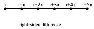
No. of nodes to be taken is calculated by
No. of nodes = p+q
where p = order of the derivative
q = order of approximation.
Here p=2 and q=4
so, no. of nodes = 2+4 = 6
4th order of approximation is given by the equation
`(del^2u)/(del x)^2` = `(af(i)+bf(i+1)+cf(i+2)+df(i+3)+ef(i+4)+gf(i+5))/(Delta x)^2` ................eq2
`af(i) = a(f(i)`
`b(f(i+1)` = `bf(i)+bΔxf′(i)+b(Δx)^2/(2!)f′′(i)+b(Δx)^3/(3!)f′′′(i)+b(Δx)^4/(4!)f′′′′(i)+b(Δx)^5/(5!)f′′′′′(i)`
`c(f(i+2)` = `cf(i)+c2Δxf′(i)+c(2Δx)^2/(2!)f′′(i)+c(2Δx)^3/(3!)f′′′(i)+c(2Δx)^4/(4!)f′′′′(i)+c(2Δx)^5/(5!)f′′′′′(i)`
`df(i+3)` = `df(i)+d3Δxf′(i)+d(3Δx)^2/(2!)f′′(i)+d(3Δx)^3/(3!)f′′′(i)+d(3Δx)^4/(4!)f′′′′(i)+d(3Δx)^5/(5!)f′′′′′(i)`
`ef(i+4)` = `ef(i)+e4Δxf′(i)+e(4Δx)^2/(2!)f′′(i)+e(4Δx)^3/(3!)f′′′(i)+e(4Δx)^4/(4!)f′′′′(i)+e(4Δx)^5/(5!)f′′′′′(i)`
`gf(i+5)` = `gf(i)+g5Δxf′(i)+g(5Δx)^2/(2!)f′′(i)+g(5Δx)^3/(3!)f′′′(i)+g(5Δx)^4/(4!)f′′′′(i)+g(5Δx)^5/(5!)f′′′′′(i)`
Taylor Table for central difference Skewed right-sided difference
| Taylor Table | ||||||
| Assumed Function | Taylor Series Expansion | |||||
| f(i) | Δxf′(i) | Δx^2f''(i) | Δx^3f'''(i) | Δx^4f''''(i) | Δx^5f'''''(i) | |
| a(i) | a | 0 | 0 | 0 | 0 | 0 |
| b(i+1) | b | b | b/2 | b/6 | b/24 | b/120 |
| c(i+2) | c | 2c | 4c/2 | 8c/6 | 16c/24 | 32c/120 |
| d(i+3) | d | 3d | 9d/2 | 27d/6 | 81d/24 | 243d/120 |
| e(1+4) | e | 4e | 16e/2 | 64e/6 | 256e/24 | 1024e/120 |
| g(i+5) | g | 5g | 25g/2 | 125g/6 | 625g/24 | 3125g/120 |
| Sum of Coefficients | 0 | 0 | 1 | 0 | 0 | 0 |
a+b+c+d+e+g=0
0+b+2c+3d+4e+5g=0
0+b/2+4/2c+9/2e+16/2e+25g/2 =1
0+b/6+8c/6+27d/6+64e/6+125g/6=0
0+b/24+16c/24+81d/24+256e/24+625g/24=0
0+b/120+32c/120+243d/120+1024e/120+3125g/120=0
From the above equations
A= [ 1 1 1 1 1 1;
0 1 2 3 4 5;
0 1/2 2 9/2 8 25/2;
0 1/6 4/3 27/6 64/6 125/6;
0 1/24 2/3 81/24 256/24 625/24;
0 1/120 16/60 243/120 1024/120 3125/120; ]
B= [0;0;1;0;0;0]
X=[A] inverse*[B]
Find the coefficients and substitute in eq1 so we will get general form 4th order of approximation for Central difference
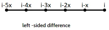
3. Skewed left-sided difference: A "skewed left" distribution is one in which the tail is on the left side.
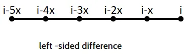
No. of nodes to be taken is calculated by
No. of nodes = p+q
where p = order of the derivative
q = order of approximation.
Here p=2 and q=4
so, no. of nodes = 2+4 = 6
4th order of approximation is given by the equation
`(del^2u)/(del x)^2` = `(af(i)+bf(i-1)+cf(i-2)+df(i-3)+ef(i+4)+gf(i-5))/(Delta x)^2` ................eq2
`af(i) = a(f(i)`
`b(f(i-1)` = `bf(i)-bΔxf′(i)+b(Δx)^2/(2!)f′′(i)-b(Δx)^3/(3!)f′′′(i)+b(Δx)^4/(4!)f′′′′(i)-b(Δx)^5/(5!)f′′′′′(i)`
`c(f(i-2)` = `cf(i)-c2Δxf′(i)+c(2Δx)^2/(2!)f′′(i)-c(2Δx)^3/(3!)f′′′(i)+c(2Δx)^4/(4!)f′′′′(i)-c(2Δx)^5/(5!)f′′′′′(i)`
`df(i-3)` = `df(i)-d3Δxf′(i)+d(3Δx)^2/(2!)f′′(i)-d(3Δx)^3/(3!)f′′′(i)+d(3Δx)^4/(4!)f′′′′(i)-d(3Δx)^5/(5!)f′′′′′(i)`
`ef(i-4)` = `ef(i)-e4Δxf′(i)+e(4Δx)^2/(2!)f′′(i)-e(4Δx)^3/(3!)f′′′(i)+e(4Δx)^4/(4!)f′′′′(i)-e(4Δx)^5/(5!)f′′′′′(i)`
`gf(i-5)` = `gf(i)-g5Δxf′(i)+g(5Δx)^2/(2!)f′′(i)-g(5Δx)^3/(3!)f′′′(i)+g(5Δx)^4/(4!)f′′′′(i)-g(5Δx)^5/(5!)f′′′′′(i)`
Taylor Table for central difference Skewed right-sided difference
| Taylor Table | ||||||
| Assumed Function | Taylor Series Expansion | |||||
| f(i) | Δxf′(i) | Δx^2f''(i) | Δx^3f'''(i) | Δx^4f''''(i) | Δx^5f'''''(i) | |
| a(i) | a | 0 | 0 | 0 | 0 | 0 |
| b(i-1) | b | -b | b/2 | -b/6 | b/24 | -b/120 |
| c(i-2) | c | -2c | 4c/2 | -8c/6 | 16c/24 | -32c/120 |
| d(i-3) | d | -3d | 9d/2 | -27d/6 | 81d/24 | -243d/120 |
| e(1-4) | e | -4e | 16e/2 | -64e/6 | 256e/24 | -1024e/120 |
| g(i-5) | g | -5g | 25g/2 | -125g/6 | 625g/24 | -3125g/120 |
| Sum of Coefficients | 0 | 0 | 1 | 0 | 0 | 0 |
a+b+c+d+e+g=0
0-b-2c-3d-4e-5g=0
0+b/2+4/2c+9/2e+16/2e+25g/2 =1
0-b/6-8c/6-27d/6-64e/6-125g/6=0
0+b/24+16c/24+81d/24+256e/24+625g/24=0
0-b/120-32c/120-243d/120-1024e/120-3125g/120=0
From the above equations
A= [ 1 1 1 1 1 1;
0 - 1 - 2 - 3 -4 - 5;
0 1/2 2 9/2 8 25/2;
0 - 1/6 -4/3 -27/6 - 64/6 -125/6;
0 1/24 2/3 81/24 256/24 625/24;
0 -1/120 - 16/60 -243/120 -1024/120 - 3125/120; ]
B= [0;0;1;0;0;0]
X=[A] inverse*[B]
Find the coefficients and substitute in eq1 so we will get general form 4th order of approximation for Central difference.
Program:
Input data
x = pi/3; x is the fixed value so using this x data as referance and computing
1. Central difference
2. Skewed right-sided difference
3. Skewed left-sided difference
dx=linspace(pi/4,pi/400,20); % Range of dx
for i=1:length(dx)
central_differencing_error(i) = central_difference_approximation(x,dx(i)); %calling function central_difference_approximation
right_side_differencing_error(i) = right_side_difference_approximation(x,dx(i)); %calling function right_side_difference_approximation
left_side_differencing_error(i) = left_side_difference_approximation(x,dx(i)); %calling function left_side_difference_approximation
end
figure(1)
loglog(dx,central_differencing_error,'color','g','linewidth',1.5)
hold on
loglog(dx,right_side_differencing_error,'color','b','linewidth',1.5)
loglog(dx,left_side_differencing_error,'color','r','linewidth',1.5)
xlabel('dx')
ylabel('Absolute Error')
legend('Central difference of 4th order','Skewed Right Sided Difference od 4th Order','Skewed Left Sided Difference of 4th Order')
title('dx Vs errors')
%Write a program that Deriving 4th order approximation of a 2nd order derivative using Taylor Table method
close all
clear all
clc
% Input data
x = pi/3;

dx=linspace(pi/4,pi/400,20); % Range of dx


for i=1:length(dx)

    central_differencing_error(i) = central_difference_approximation(x,dx(i)); %calling function central_difference_approximation
     right_side_differencing_error(i) = right_side_difference_approximation(x,dx(i)); %calling function right_side_difference_approximation
     left_side_differencing_error(i) = left_side_difference_approximation(x,dx(i)); %calling function left_side_difference_approximation

end

figure(1)

loglog(dx,central_differencing_error,'color','g','linewidth',1.5)
hold on
loglog(dx,right_side_differencing_error,'color','b','linewidth',1.5)
loglog(dx,left_side_differencing_error,'color','r','linewidth',1.5)
xlabel('dx')
ylabel('Absolute Error')
legend('Central difference of 4th order','Skewed Right Sided Difference od 4th Order','Skewed Left Sided Difference of 4th Order')
title('dx Vs errors')
Functions: here we have 3 different function for 3 schems
all function have same procedure
1. finding the 2nd order Analytical derivative.
2. 4th order approximations of the second-order derivative Using 3 different schemes.
3. For finding the coefficient have used the formula X= inv(A)*B;
4. Substitute X values in Taylor series and find the 4th order approximation of a 2nd order derivative using Taylor Table method.
1. Central difference
 function out = central_difference_approximation(x,dx) %Function for central_difference_approximation
% Given function f(x)= exp(x)*cos(x)
%Analytical derivative for the function f(x ) is f'(x). which looks f(x)= u*v
% f'(x) = uv'+u'v
% f'(x) = exp(x)*-sin(x)+cos(x)*exp(x) = exp(x)*(cos(x)-sin(x))
% f''(x) = exp(x)*(-sin(x)-cos(x))+ exp(x)*(cos(x)-sin(x))
% f''(x) = exp(x)*((-sin(x)-cos(x))+(cos(x)-sin(x))= (-2*(exp(x)*sin(x)))
analytical_derivative = (-2*(exp(x)*sin(x)));

%4th order approximations of the second-order derivative Using Central differencing
%From the tabel

A= [1 1 1 1 1;
    -2 -1 0 1 2;
    4/2 1/2 0 1/2 4/2;
    -8/6 -1/6 0 1/6 8/6;
    16/24 1/24 0 1/24 16/24];
B= [0;
    0;
    1;
    0;
    0];
%For finding the coefficient have used the formula
X= inv(A)*B;

% Substitute X values in Taylor series
%(del^2u)/(del x)^2= f''(x) = `a(f(i−2)+bf(i−1)+cf(i)+df(i+1)+ef(i+2))/(Delta x)^2` ................eq1
%f''(x) = `-0.0833(f(i−2)+1.3333f(i−1)-2.5000f(i)+ 1.3333f(i+1)-0.0833f(i+2))/(Delta x)^2` ................eq1

term1 = (X(1))*(exp(x-(2*dx)))*(cos(x-(2*dx)));
term2 = (X(2))*(exp(x-dx))*(cos(x-dx));
term3 = (X(3))*(exp(x))*(cos(x));
term4 = (X(4))*(exp(x+dx))*(cos(x+dx));
term5 = (X(5))*(exp(x+(2*dx)))*(cos(x+(2*dx)));

% 2nd order central difference
central_difference = (term1 + term2 + term3 + term4 + term5)/(dx)^2;


error = abs(central_difference-analytical_derivative);

out = error;

 end
2. Skewed right-sided difference
 function out = right_side_difference_approximation(x,dx) %Function for central_difference_approximation
% Given function f(x)= exp(x)*cos(x)
%Analytical derivative for the function f(x ) is f'(x). which looks f(x)= u*v
% f'(x) = uv'+u'v
% f'(x) = exp(x)*-sin(x)+cos(x)*exp(x) = exp(x)*(cos(x)-sin(x))
% f''(x) = exp(x)*(-sin(x)-cos(x))+ exp(x)*(cos(x)-sin(x))
% f''(x) = exp(x)*((-sin(x)-cos(x))+(cos(x)-sin(x))= (-2*(exp(x)*sin(x)))
analytical_derivative = (-2*(exp(x)*sin(x)));

%4th order approximations of the second-order derivative Using Central differencing
%From the tabel


A= [1 1 1 1 1 1;
    0 1 2 3 4 5;
    0 1/2 4/2 9/2 16/2 25/2;
    0 1/6 8/6 27/6 64/6 125/6;
    0 1/24 16/24 81/24 256/24 625/24;
    0 1/120 32/120 243/120 1024/120 3125/120];
B= [0;
    0;
    1;
    0;
    0;
    0];
%For finding the coefficient have used the formula
X= inv(A)*B;


% Substitute X values in Taylor series
%   `(del^2u)/(del x)^2` = `(af(i)+bf(i+1)+cf(i+2)+df(i+3)+ef(i+4)+gf(i+5))/(Delta x)^2` ................eq2

term1 = (X(1))*(exp(x))*(cos(x));
term2 = (X(2))*(exp(x+dx))*(cos(x+dx));
term3 = (X(3))*(exp(x+(2*dx)))*(cos(x+2*dx));
term4 = (X(4))*(exp(x+(3*dx)))*(cos(x+3*dx));
term5 = (X(5))*(exp(x+(4*dx)))*(cos(x+4*dx));
term6 = (X(6))*(exp(x+(5*dx)))*(cos(x+5*dx));

% 2nd order right_side_differencing
right_side_differencing = (term1 + term2 + term3 + term4 + term5 + term6)/(dx)^2;

error = abs(right_side_differencing-analytical_derivative);

out = error;

 end
3. Skewed left-sided difference
 function out = left_side_difference_approximation(x,dx) %Function for central_difference_approximation
% Given function f(x)= exp(x)*cos(x)
%Analytical derivative for the function f(x ) is f'(x). which looks f(x)= u*v
% f'(x) = uv'+u'v
% f'(x) = exp(x)*-sin(x)+cos(x)*exp(x) = exp(x)*(cos(x)-sin(x))
% f''(x) = exp(x)*(-sin(x)-cos(x))+ exp(x)*(cos(x)-sin(x))
% f''(x) = exp(x)*((-sin(x)-cos(x))+(cos(x)-sin(x))= (-2*(exp(x)*sin(x)))
analytical_derivative = (-2*(exp(x)*sin(x)));

%4th order approximations of the second-order derivative Using Central differencing
%From the tabel


A= [1 1 1 1 1 1;
    0 -1 -2 -3 -4 -5;
    0 1/2 4/2 9/2 16/2 25/2;
    0 -1/6 -8/6 -27/6 -64/6 -125/6;
    0 1/24 16/24 81/24 256/24 625/24;
    0 -1/120 -32/120 -243/120 -1024/120 -3125/120];
B= [0;
    0;
    1;
    0;
    0;
    0];
%For finding the coefficient  have used the formula
X= inv(A)*B;


% Substitute X values in Taylor series
% `(del^2u)/(del x)^2` = `(af(i)+bf(i-1)+cf(i-2)+df(i-3)+ef(i+4)+gf(i-5))/(Delta x)^2` ................eq2

term1 = (X(1))*(exp(x))*(cos(x));
term2 = (X(2))*(exp(x-dx))*(cos(x-dx));
term3 = (X(3))*(exp(x-(2*dx)))*(cos(x-2*dx));
term4 = (X(4))*(exp(x-(3*dx)))*(cos(x-3*dx));
term5 = (X(5))*(exp(x-(4*dx)))*(cos(x-4*dx));
term6 = (X(6))*(exp(x-(5*dx)))*(cos(x-5*dx));

% 2nd order left_side_differencing
left_side_differencing = (term1 + term2 + term3 + term4 + term5 + term6)/(dx)^2;


error = abs(left_side_differencing-analytical_derivative);

out = error;

 end
Results:
Derive the Central difference, Skewed right-sided difference and Skewed left-sided difference 4th order approximations of the second-order derivative is done.
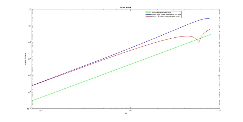
1. From the plot we can say central differencing will give the less error compared to Skewed right-sided difference and Skewed left-sided difference. central differencing will be calculated based on both the directions.
2. Skewed right-sided difference and Skewed left-sided difference are same as dx tends to x we can see instability in Skewed left-sided difference.
3. central differencing can use only if we have mid referance point. Skewed right-sided difference and Skewed left-sided difference can used for +ve and -ve direction.
In your own words, describe why a skewed scheme is useful? What can a skewed scheme do that a CD scheme cannot?
central differencing can use only if we have mid referance point. Skewed right-sided difference and Skewed left-sided difference can used for +ve and -ve direction. depending on the direction of information flow.