theory is described in word file attached below. please refer it
close all
clear all
clc
% ANALYTICAL FUNCTION, f(x)=exp(x)*cos(x)
%ANALYTICAL DERIVATIVE
%f''(x) = -2*exp(x)*sin(x)
x =pi/3; % FOR x = pi/3 assumed
y2 = -2*exp(x)*sin(x) % analytical second order derivative of function f(x)
% numerical method to solve the problem
dx=linspace(pi/4000,pi/40,40); % creating nodes on x axis
for i=1:40
%skewed left-sided differencing used to find 2nd order derivative[y2]
% y2=(3.75*f(i)-12.8333*f(i-1)+17.8333*f(i-2)-13*f(i-3)+5.0833*f(i-4)-0.8333*f(i-5)/(dx^2) as calculated in theory of this report
y2l(i) = (3.75*(exp(x)*cos(x)) - 12.8333*(exp(x-dx(i))*cos(x-dx(i))) + 17.8333*(exp(x-2*dx(i))*cos(x-2*dx(i))) - 13*(exp(x-3*dx(i))*cos(x-3*dx(i))) + 5.0833*(exp(x-4*dx(i))*cos(x-4*dx(i))) - 0.8333*(exp(x-5*dx(i))*cos(x-5*dx(i))))/(dx(i)^2); %skewed left-sided differencing for 2nd order derivative
% central differencing used to find 2nd order derivative[y2]
% y2=(-0.0833*f(i-2) + 1.3333*f(i-1) - 2.5*f(i) + 1.3333*f(i+1) - 0.0833*f(i+2))/(dx^2) as calculated in theory of this report
y2c(i) = (-0.0833*(exp(x-2*dx(i))*cos(x-2*dx(i))) + 1.3333*(exp(x-dx(i))*cos(x-dx(i))) - 2.5*(exp(x)*cos(x)) + 1.3333*((exp(x+dx(i))*cos(x+dx(i)))) - 0.0833*(exp(x+2*dx(i))*cos(x+2*dx(i))))/(dx(i)^2); %central differencing for 2nd order derivative
%skewed right-sided differencing used to find 2nd order derivative[y2]
% y2 = (3.75*f(i)-12.8333*f(i+1)+17.8333*f(i+2)-13*f(i+3)+5.0833*f(i+4)-0.8333*f(i+5)/(dx^2) as calculated in theory of this report
y2r(i) = (3.75*(exp(x)*cos(x)) - 12.8333*(exp(x+dx(i))*cos(x+dx(i))) + 17.8333*(exp(x+2*dx(i))*cos(x+2*dx(i))) - 13*(exp(x+3*dx(i))*cos(x+3*dx(i))) + 5.0833*(exp(x+4*dx(i))*cos(x+4*dx(i))) - 0.8333*(exp(x+5*dx(i))*cos(x+5*dx(i))))/(dx(i)^2); %skewed right-sided differencing for 2nd order derivative
%calculating errors
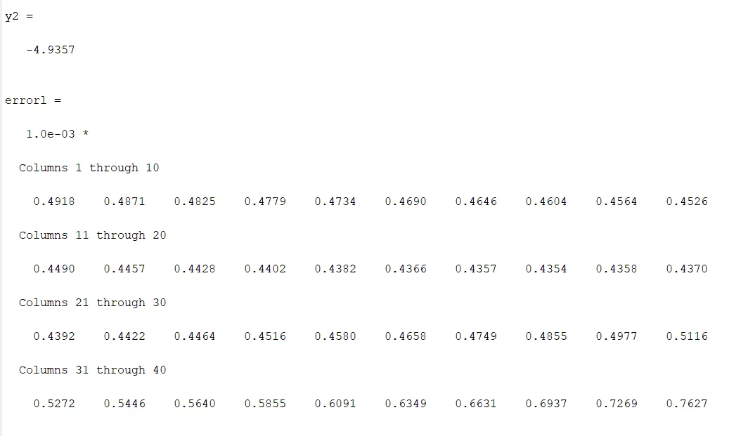
errorl(i) = abs(y2l(i) - y2); %error for skewed left-sided differencing wrt analytical value
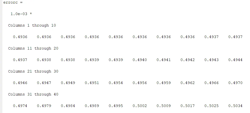
errorc(i) = abs(y2c(i) - y2); %error for central differencing wrt analytical value
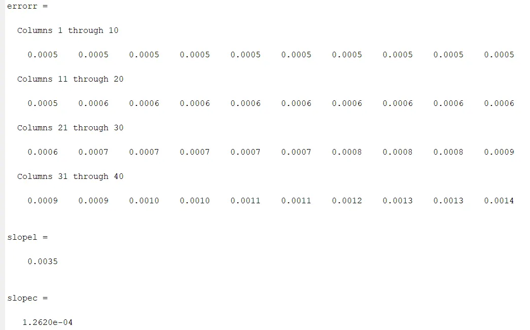
errorr(i) = abs(y2r(i) - y2); %error for skewed right-sided differencing wrt analytical value
end
display(errorl)
display(errorc)
display(errorr)
% display(dx)
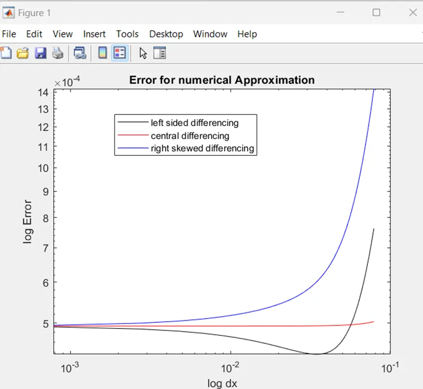
figure(1)
loglog(dx,errorl, 'color','k')
hold on
loglog(dx,errorc,'color','r')
loglog(dx,errorr,'color','b')
xlabel('log dx')
ylabel('log Error')
title("Error for numerical Approximation")
legend("left sided differencing","central differencing","right skewed differencing")
% calculating slopes
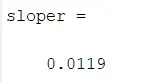
slopel = mean(diff(errorl)./diff(dx)) % as the curves are not linear, we need to find mean for left skewed differencing
slopec = mean(diff(errorc)./diff(dx)) % as the curves are not linear, we need to find mean for central differencing
sloper = mean(diff(errorr)./diff(dx)) % as the curves are not linear, we need to find mean for right skewed differencing
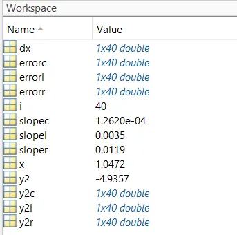
OUTPUT:
CONCLUSION:
1. We can see the from the plot that the central differencing is almost linear with very less deviation in slopes or error deviation from analytical value at each node on x thus central differencing satisfies more towards analytical value than others.
2. Left sided differencing shows wide deviation in slopes or error deviation from analytical value as we move far from the prime node x=I than right sided differencing
In your own words, describe why a skewed scheme is useful? What can a skewed scheme do that a CD scheme cannot?
Answer: there are so many physical problems where the dependent variable varies in one direction only wrt independent variable like flow of water in open channel or heat flow through a bar in one direction when it gets contacted with a hot wall.
Central differencing is usefull when water flows in pipe or heat source generating heat in a rod in both direction.