Week 3.5 - Deriving 4th order approximation of a 2nd order derivative using Taylor Table method

Deriving 4th order approximation of a 2nd order derivative using the Taylor Table method

Derive the following 4th-order approximations of the second-order derivative.

1. Central difference

2. Skewed right-sided difference

3. Skewed left-sided difference

After deriving these schemes, prove that your skewed schemes are fourth-order accurate i.e the thumb rule is given in HINT (ii).

Once you have done this, write a program in Matlab to evaluate the second-order derivative of the analytical function exp(x)*cos(x) and compare it with the 3 numerical approximations that you have derived.

Provide a plot that compares the absolute error between the above-mentioned schemes

In your own words, describe why a skewed scheme is useful. What can a skewed scheme do that a Central Difference scheme cannot?

HINT :

i) The order of accuracy P = Number of nodes in the stencil N - order of derivative Q + 1 for symmetric/central schemes

ii) The order of accuracy P = Number of nodes in the stencil N - order of derivative Q for one-sided/skewed schemes

iii) Solve the system of equations using the matrix inversion method in Matlab to obtain the Taylor table coefficients and use them directly in the numerical approximation statements to avoid input errors.

Introduction

Central difference

The central difference is a numerical method used to approximate the derivative of a function at a specific point. It is a finite difference method that involves evaluating the function at two neighboring points and then taking the difference of their function values. The central difference method provides a more accurate approximation of the derivative compared to forward or backward difference methods because it takes into account information from both sides of the point.

It is commonly used in numerical analysis and computational methods when an analytical expression for the derivative is not available or when dealing with discrete data points. The central difference is particularly useful for calculating derivatives in cases of discrete and noisy data, where analytical methods might not be feasible or accurate enough.

The order of accuracy P = Number of nodes in the stencil N - order of derivative Q + 1 for symmetric/central schemes

N=P+Q-1

N=4+2-1

N=5

`(d^2f)/dx^2=af(i-2)+bf(i-1)+cf(i)+df(i+1)+ef(i+2)`

• a, b, c, d, and e are constants determined by the function and its derivatives.
• f(i) represents the value of the function f(x) at the point i.
• The terms f(i-2), f(i-1), f(i), f(i+1), and f(i+2) represent the function values at points i-2, i-1, i, i+1, and i+2, respectively.
• The Taylor series expansion represents an approximation of the nth derivative of the function f(x) using the function values at multiple points around i. The coefficients a, b, c, d, and e are chosen in such a way that the approximation provides an accurate representation of the 2nd derivative. The Taylor series expansion becomes more accurate as the number of terms considered increases, with higher-order approximations providing better accuracy.

Taylor series expansion for the above equation:

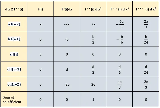
Converting the above table to matrix format and solving each element

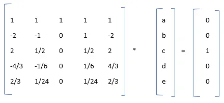
we got a=-0.0834, b=1.34, c=-2.5, d=1.34, e=-0.0834

SKEWED RIGHT-SIDED DIFFERENCE

The Skewed Right-Sided Difference is a numerical approximation method that is used to find a function's derivatives at a specific place. This technique, which is especially useful when working with asymmetric data or functions with steep slopes, extends the fundamental finite difference method.

The order of accuracy P = Number of nodes in the stencil N - order of derivative Q for one-sided/skewed schemes

N=P+Q

N=4+2

N=6

`(d^2f)/dx^2=a.f(i)+b.f(i+1)+c.f(i+2)+d.f(i+3)+e.f(i+4)+f.f(i+f)`

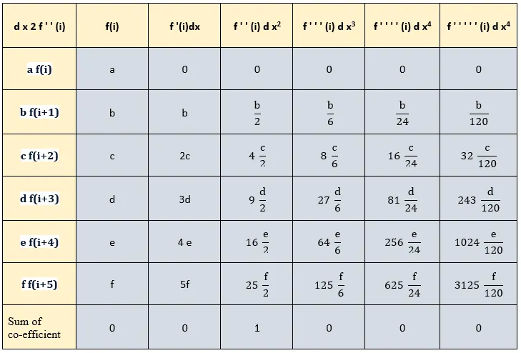
Converting the above table to matrix format and solving each element

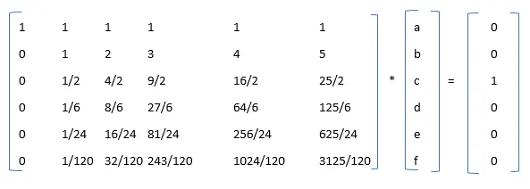
we got a=3.75, b=-12.84, c=17.834, d=-13, e=5.0834, f=-0.0834

SKEWED LEFT-SIDED DIFFERENCE

The Skewed Left-Sided Difference is another numerical approximation method used to ascertain a function's derivatives at a specific position. Similar to the Skewed Right-Sided Difference, it is an extension of the conventional finite difference method and is particularly beneficial when dealing with asymmetric data or functions with steep slopes.

The order of accuracy P = Number of nodes in the stencil N - order of derivative Q for one-sided/skewed schemes

N=P+Q

N=4+2

N=6

`(d^2f)/dx^2=a.f(i-5)+b.f(i-4)+c.f(i-3)+d.f(i-2)+e.f(i-1)+f.f(i)`

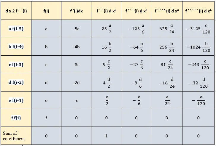
Converting the above table to matrix format and solving each element

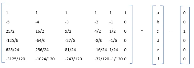
we got a=-0.0834, b=5.0834, c=-13, d=17.834, e=-12.84, f=3.75

Program

clc
clear all
close all

% Define the value of x
x = pi/4;

% Define the range of dx
dx = linspace(pi/20, pi/400, 40);

% Initialize arrays to store results

central_error = zeros(1, length(dx));

forward_error = zeros(1, length(dx));

backward_error = zeros(1, length(dx));

% Exact derivative of the function exp(x)*cos(x)

exact_derivative = -2 * exp(x) * sin(x);

for i = 1:length(dx)
   
    % Calculate errors for each approximation scheme
   
    [central_diff, forward_diff, backward_diff] = taylor_table_scheme(x, dx(i));

    % Compute errors for each scheme
   
    central_error(i) = abs(exact_derivative - central_diff);
   
    forward_error(i) = abs(exact_derivative - forward_diff);
   
    backward_error(i) = abs(exact_derivative - backward_diff);

end

% Plot the errors

figure(1)

plot(dx, central_error, 'r-')

hold on 

plot(dx, forward_error, 'b-')

hold on

plot(dx, backward_error, 'g-')

xlabel('dx')

ylabel('error')

legend('Central difference scheme', 'Forward difference scheme', 'Backward difference 
scheme')

title('Comparison of errors for a 2nd order derivative 4th order approximation using different approximation schemes')

% Plot the errors on a log-log scale

figure(2)

loglog(dx, central_error, 'r-')

hold on 

loglog(dx, forward_error, 'b-')

hold on

loglog(dx, backward_error, 'g-')

xlabel('log(dx)')

ylabel('log(error)')

legend('Central difference scheme', 'Forward difference scheme', 'Backward difference scheme')

title('Comparison of errors for a 2nd order derivative 4th order approximation using different approximation schemes (on log-log scale)')

% Function to calculate numerical derivatives using various schemes

function [central_diff, forward_diff, backward_diff] = taylor_table_scheme(x, dx)

    % Central difference scheme
    
    central_diff = ((-1 * exp(x + (2 * dx)) * cos(x + (2 * dx))) + (16 * exp(x + dx) * cos(x + dx)) + ...
        (-30 * exp(x) * cos(x)) + (16 * exp(x - dx) * cos(x - dx)) + (-1 * exp(x - (2 * dx)) * cos(x - (2 * dx)))) / (12 * (dx^2));

    % Skewed forward difference scheme
    
    forward_diff = ((45 * exp(x) * cos(x)) + (-154 * exp(x + dx) * cos(x + dx)) + (214 * exp(x + (2 * dx)) * cos(x + (2 * dx))) + ...
        (-156 * exp(x + (3 * dx)) * cos(x + (3 * dx))) + (61 * exp(x + (4 * dx)) * cos(x + (4 * dx))) + (-10 * exp(x + (5 * dx)) * cos(x + (5 * dx)) )) / (12 * (dx^2));

    % Skewed backward difference scheme
    
    backward_diff = ((45 * exp(x) * cos(x)) + (-154 * exp(x - dx) * cos(x - dx)) + (214 * exp(x - (2 * dx)) * cos(x - (2 * dx))) + ...
        (-156 * exp(x - (3 * dx)) * cos(x - (3 * dx))) + (61 * exp(x - (4 * dx)) * cos(x - (4 * dx))) + (-10 * exp(x - (5 * dx)) * cos(x - (5 * dx)) )) / (12 * (dx^2));

end

Result

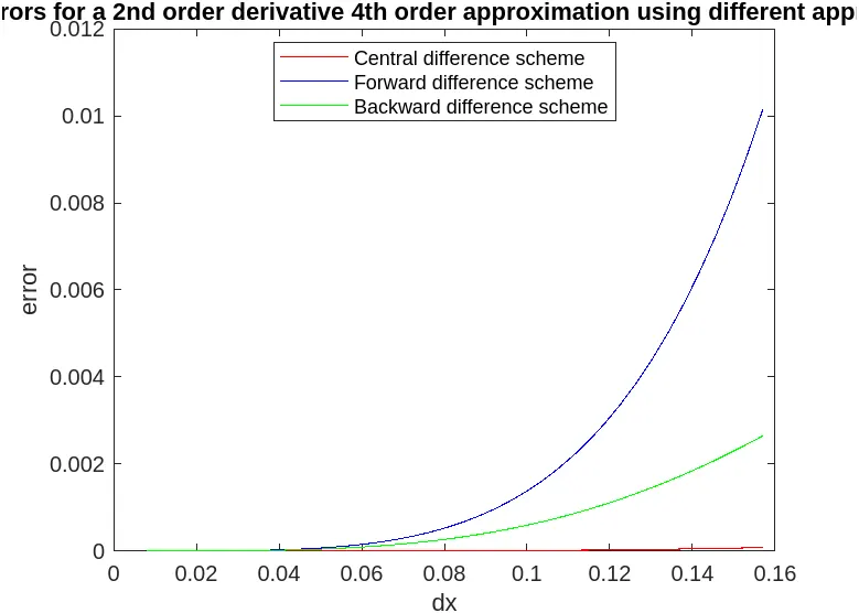
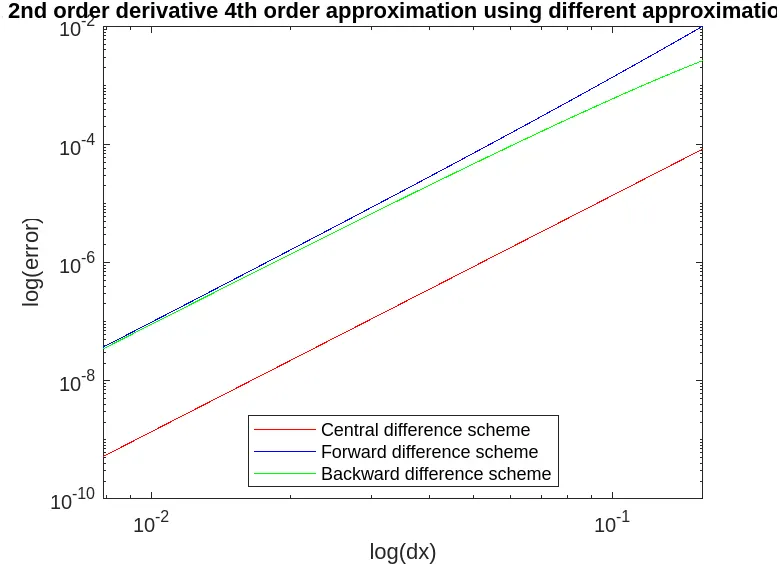
The usage of Skewed Difference schemes in numerical differentiation gives considerable advantages over the traditional Central Difference scheme. Skewed Difference schemes, which allow for uneven steps and cause shifts in the grid points, increase accuracy in functions with extreme asymmetries or steep gradients. They offer versatility and improved resolution close to important sites, and they are excellent at managing data with unpredictable spacing and boundary conditions. Skewed Difference schemes are highly helpful in simulations and scientific computations since they reduce oscillations and numerical dissipation as well.

Skewed difference schemes will remain crucial tools in many scientific and engineering applications as numerical techniques develop and create increasingly precise and trustworthy approximations. They can handle difficult situations and offer longer-lasting answers for the benefit of academics and practitioners. Skewed difference schemes provide a realistic route to greater precision and efficiency in the pursuit of exact numerical differentiation.