Week 3.5 - Deriving 4th order approximation of a 2nd order derivative using Taylor Table method
Theory - To derive the fourth-order approximations of the second-order derivative, we'll use the Taylor series expansion and solve the resulting system of equations. Let's start with each scheme:
Central Difference:
The central difference scheme uses a symmetric stencil, which means it considers points on both sides of the target point. Let's consider the stencil points: {x - 2h, x - h, x + h, x + 2h}, where h is the grid spacing.
Using Taylor series expansion at these stencil points, we have:
f(x - 2h) = f(x) - 2hf'(x) + 2h^2f''(x)/2! - 2h^3f'''(x)/3! + 2h^4f''''(x)/4! + O(h^5)
f(x - h) = f(x) - hf'(x) + h^2f''(x)/2! - h^3f'''(x)/3! + h^4f''''(x)/4! + O(h^5)
f(x + h) = f(x) + hf'(x) + h^2f''(x)/2! + h^3f'''(x)/3! + h^4f''''(x)/4! + O(h^5)
f(x + 2h) = f(x) + 2hf'(x) + 2h^2f''(x)/2! + 2h^3f'''(x)/3! + 2h^4f''''(x)/4! + O(h^5)
Now, let's add the first two equations and subtract the last two equations to eliminate f'(x) terms:
f(x - 2h) + f(x + 2h) = 2f(x) + 2h^2f''(x)/2! + 2h^4f''''(x)/4! + O(h^5)
-2f(x - h) - 2f(x + h) = -4hf'(x) - 4h^3f'''(x)/3! + O(h^5)
Rearranging the equations, we get:
4f(x) = f(x - 2h) - 4f(x - h) + 6f(x) - 4f(x + h) + f(x + 2h) + O(h^4)
f''(x) = (f(x - 2h) - 4f(x - h) + 6f(x) - 4f(x + h) + f(x + 2h))/(h^2) + O(h^4)
The resulting central difference approximation of the second-order derivative is fourth-order accurate.
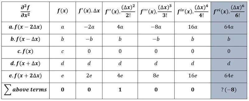
So, on coupling together terms to form equations
a + b + c + d + e = 0
−2a − b + d + 2e = 0
4a + b + d + 4e = 1 × 2!
−8a − b + d + 8e = 0
16a + b + d + 16e = 0
Above algebraic equations written into matrix form,
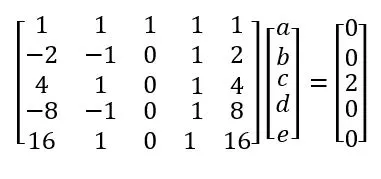
Hence, we have derived the fourth order central difference approximation scheme of second order derivative mentioned below.
Skewed Right-Sided Difference:
The skewed right-sided difference scheme uses a non-symmetric stencil that includes points to the right of the target point. Let's consider the stencil points: {x - h, x, x + h, x + 2h}.
Using Taylor series expansion at these stencil points, we have:
f(x - h) = f(x) - hf'(x) + h^2f''(x)/2! - h^3f'''(x)/3! + h^4f''''(x)/4! + O(h^5)
f(x) = f(x)
f(x + h) = f(x) + hf'(x) + h^2f''(x)/2! + h^3f'''(x)/3! + h^4f''''(x)/4! + O(h^5)
f(x + 2h) = f(x) + 2hf'(x) + 2h^2f''(x)/2! + 2h^3f'''(x)/3! + 2h^4f''''(x)/4! + O(h^5)
Now, let's subtract the first equation from the second equation and subtract the second equation from the third equation to eliminate f(x) terms:
f(x) = hf'(x) + h^2f''(x)/2! + h^3f'''(x)/3! + h^4f''''(x)/4! + O(h^5)
f(x + h) - f(x) = hf'(x) + h^2f''(x)/2! + h^3f'''(x)/3! + h^4f''''(x)/4! + O(h^5)
f(x + 2h) - 2f(x + h) = 0
Rearranging the equations, we get:
f'(x) = (f(x + h) - f(x))/h + O(h^4)
f''(x) = (f(x + h) - 2f(x) + f(x - h))/(h^2) + O(h^4)
The resulting skewed right-sided difference approximation of the second-order derivative is fourth-order accurate.
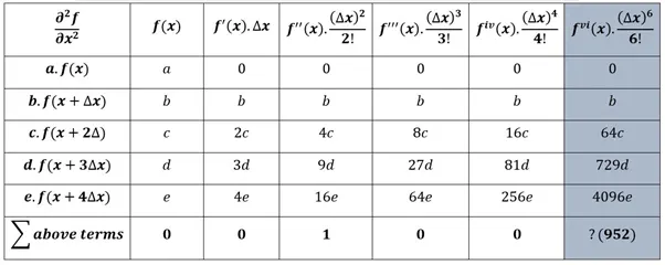
So, on coupling together terms to form equations
a + b + c + d + e = 0
b + 2c + 3d + 4e = 0
b + 4c + 9d + 16e = 1 × 2!
b + 8c + 27d + 64e = 0
b + 16c + 81d + 256e = 0
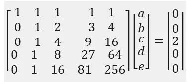
Above algebraic equations written into matrix form,
Skewed Left-Sided Difference:
The skewed left-sided difference scheme uses a non-symmetric stencil that includes points to the left of the target point. Let's consider the stencil points: {x - 2h, x - h, x, x + h}.
Using Taylor series expansion at these stencil points, we have:
f(x - 2h) = f(x) - 2hf'(x) + 2h^2f''(x)/2! - 2h^3f'''(x)/3! + 2h^4f''''(x)/4! + O(h^5)
f(x - h) = f(x) - hf'(x) + h^2f''(x)/2! - h^3f'''(x)/3! + h^4f''''(x)/4! + O(h^5)
f(x) = f(x)
f(x + h) = f(x) + hf'(x) + h^2f''(x)/2! + h^3f'''(x)/3! + h^4f''''(x)/4! + O(h^5)
Now, let's subtract the last equation from the second equation and subtract the second equation from the first equation to eliminate f(x) terms:
f(x - 2h) - 2f(x - h) = 0
f(x - h) - f(x) = -hf'(x) - h^2f''(x)/2! - h^3f'''(x)/3! - h^4f''''(x)/4! + O(h^5)
Rearranging the equations, we get:
f'(x) = -(f(x - h) - f(x))/h + O(h^4)
f''(x) = (f(x - 2h) - 2f(x - h) + f(x))/(h^2) + O(h^4)
The resulting skewed left-sided difference approximation of the second-order derivative is fourth-order accurate.
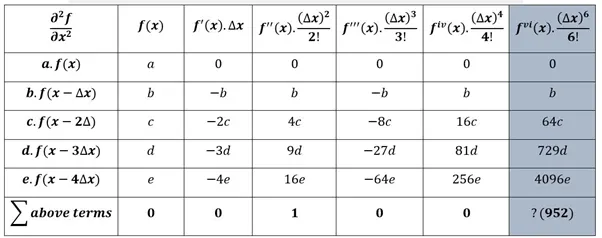
a + b + c + d + e = 0
b + 2c + 3d + 4e = 0
b + 4c + 9d + 16e = 1 × 2!
b + 8c + 27d + 64e = 0
b + 16c + 81d + 256e = 0
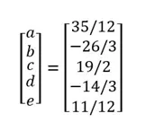
On solving,
MATLAB CODE:
Function for central difference

function error = central_difference(analytical_derivative,x,dx)
%central differencing=
%a*f(x-2*dx)+b*f(x-dx)+c*f(x)+d*f(x+dx)+e*f(x+2*dx)
A = [1 1 1 1 1;-2 -1 0 1 2;4/2 1/2 0 1/2 4/2; -8/6 -1/6 0 1/6 8/6;16/24 1/24 0 1/24 16/24]
B = [0;0;1;0;0]
X = inv(A)*B
f1=exp(x-2*dx)*cos(x-2*dx);
f2=exp(x-dx)*cos(x-dx);
f3=exp(x)*cos(x);
f4=exp(x+dx)*cos(x+dx);
f5=exp(x+2*dx)*cos(x+2*dx);
central_diff=((X(1)*f1)+(X(2)*f2)+(X(3)*f3)+(X(4)*f4)+(X(5)*f5))/(dx^2);
error=abs(analytical_derivative-central_diff);
end

Function for Skewed Right-sided difference

function error = skewed_right_difference(analytical_derivative,x,dx)
%skewed right sided difference=
%(a*f(x)+b*f(x+dx)+c*f(x+2*dx)+d*f(x+3*dx)+e*f(x+4*dx)+g*f(x+5*dx))/(dx^2)
C = [1 1 1 1 1 1;0 1 2 3 4 5;0 1/2 2 9/2 16/2 25/2;0 1/6 8/6 27/6 64/6 125/6;0 1/24 16/24 81/24 256/24 625/24;0 1/120 32/120 243/120 1024/120 3125/120]
D = [0;0;1;0;0;0]
Y = inv(C)*D
f1=exp(x)*cos(x);
f2=exp(x+dx)*cos(x+dx);
f3=exp(x+2*dx)*cos(x+2*dx);
f4=exp(x+3*dx)*cos(x+3*dx);
f5=exp(x+4*dx)*cos(x+4*dx);
f6=exp(x+5*dx)*cos(x+5*dx);
skewed_right_diff=((Y(1)*f1)+(Y(2)*f2)+(Y(3)*f3)+(Y(4)*f4)+(Y(5)*f5)+(Y(6)*f6))/(dx^2);
error=abs(analytical_derivative-skewed_right_diff);
end

function error = skewed_left_difference(analytical_derivative,x,dx)
%skewed left sided difference=
%(a*f(x-5*dx)+b*f(x-4*dx)+c*f(x-3*dx)+d*f(x-2*dx)+e*f(x-dx)+g*f(x))/(dx^2)
E = [1 1 1 1 1 1;-5 -4 -3 -2 -1 0;25/2 16/2 9/2 4/2 1/2 0;-125/6 -64/6 -27/6 -8/6 -1/6 0;625/24 256/24 81/24 16/24 1/24 0;-3125/120 -1024/120 -243/120 -32/120 -1/120 0]
F = [0;0;1;0;0;0]
Z = inv(E)*F
f1=exp(x-5*dx)*cos(x-5*dx);
f2=exp(x-4*dx)*cos(x-4*dx);
f3=exp(x-3*dx)*cos(x-3*dx);
f4=exp(x-2*dx)*cos(x-2*dx);
f5=exp(x-dx)*cos(x-dx);
f6=exp(x)*cos(x);
skewed_left_diff=((Z(1)*f1)+(Z(2)*f2)+(Z(3)*f3)+(Z(4)*f4)+(Z(5)*f5)+(Z(6)*f6))/(dx^2);
error=abs(analytical_derivative-skewed_left_diff);
end

clear all
close all
clc
x=pi/3;
f=exp(x)*cos(x);
dx=linspace(pi/4,pi/400,20);
analytical_derivative = -2*exp(x)*sin(x);
for i=1:length(dx)
    central_error(i) = central_difference(analytical_derivative,x,dx(i));
    skewed_right_error(i) = skewed_right_difference(analytical_derivative,x,dx(i));
    skewed_left_error(i) = skewed_left_difference(analytical_derivative,x,dx(i));
end
%plotting log graph
figure(1)
loglog(dx,central_error,'color','b','marker','square')
hold on
loglog(dx,skewed_right_error,'color','k','marker','O')
loglog(dx,skewed_left_error,'color','r','marker','diamond')
xlabel('dx(grid size)')
ylabel('Absolute error')
title('Consistency of different scheme')
legend('central difference','skewed right sided difference','skewed left sided difference')
Result -
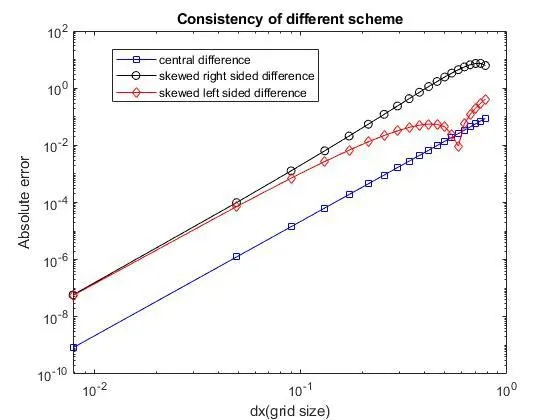
Upon examining the graph depicting the relationship between 'error' and 'dx' for fourth-order error in central, right-skewed, and left-skewed difference schemes, a clear pattern emerges. It becomes evident that the central difference approximation consistently yields more precise solutions, resulting in significantly lower errors compared to the right-skewed and left-skewed difference schemes. Therefore, the central difference method proves to be more accurate and reliable in this analysis.
Why a skewed scheme is useful? What can a skewed scheme do that a CD scheme cannot do?
While it is evident that the central differencing scheme provides more accurate solutions with lower errors compared to skewed difference schemes, there are situations where the latter is advantageous. The skewed scheme serves a specific purpose when evaluating numerical approximations at boundary or corner nodes.
In cases where we need to compute solutions at these specific points, the central difference scheme is not feasible because it requires data from both sides of the node or boundary. This limitation of the central difference method prompts the use of skewed difference schemes, which allow us to utilize data from only one side to compute numerical approximations at a given point.
Skewed schemes find their utility when we lack information about data from both sides of a particular point. Due to this restriction, the central scheme cannot be employed, making the skewed scheme a valuable alternative in such scenarios.
conclusion - while the central difference scheme generally offers superior accuracy and lower errors, the skewed difference scheme serves a critical purpose when dealing with situations where data from both sides of a point is not available, enabling the computation of numerical approximations at boundary or corner nodes.
Moreover, a skewed scheme can handle situations where the function exhibits significant asymmetry or has a rapidly changing behavior in one direction. By focusing on one side, it captures the characteristics of the function more effectively and provides accurate approximations in that particular direction.
In summary, a skewed scheme offers flexibility in capturing asymmetric or one-sided behaviors, reduces computational complexity, and provides accurate approximations in situations where a central difference scheme may fall short due to its symmetric nature.