Week 3.5 - Deriving 4th order approximation of a 2nd order derivative using Taylor Table method

Aim:

1. To derive 4^th order approximation for the 2^nd order derivative of the function: exp(x)*cos(x) with central difference, skewed right sided and skewed left sided difference method.
2. To write a matlab code to calculate the 2^nd order derivate of the analytical function and compare it with the 3 numerical approximations mentioned above.
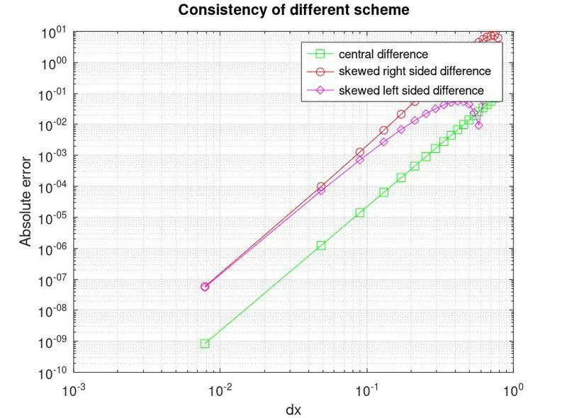
3. Provide a plot that compares absolute error between the above-mentioned schemes.
4. Explain why skewed scheme is useful? What can a skewed scheme do that CD cannot do?

Answer:

1. Let find the number of nodes required for the skewed and central difference scheme:

• For right and left sided skewed scheme:

P=N-Q

• For central difference scheme:

P=N-Q+1

Where,

P= Order of accuracy

N= Number of nodes in stencil

Q= Order of derivative

Hence, The number of nodes for left and right sided skewed schemes will be: N= 2+4= 6

And for central difference scheme N=4+2-1=5

Taylor series general equation: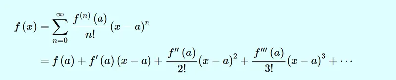

2. Let’s write the formula for the 4^th order approximation of the 2^nd order derivative for the skewed right sided and left sided scheme:
3. Right sided skewed scheme:

∆x² (d²u/dx²) = af(i)+bf(i+1)+cf(i+2)+df(i+3)+ef(i+4)+gf(i+5)

The table used for right sided skewed scheme with 6 number of nodes:

	F(i)	∆xf’(i)	∆x2f’’(i)	∆x3f’’’(i)	∆x4f’’’’(i)	∆x5f’’’’’(i)
Af(i)	A	0	0	0	0	0
Bf(i+1)	B	B	b/2	b/6	b/24	b/120
Cf(i+2)	C	2c	4c/2	8c/6	16c/24	32c/120
Df(i+3)	D	3d	9d/2	27d/6	81d/24	243d/120
Ef(i+4)	E	4e	16e/2	64e/6	256e/24	1024e/120
Gf(i+5)	g	5g	25g/2	125g/6	625g/24	3125g/120
Sum	0	0	1	0	0	0

Putting it in matrix form:

1 1 1 1 1 1 a 0

0 1 2 3 4 5 b 0

0 ½ 4/2 9/2 16/2 25/2 x c = 1

0 1/6 8/6 27/6 64/6 152/6 d 0

0 1/24 16/24 81/24 256/24 625/120 e 0

0 1/120 32/120 243/120 1024/120 3125/120 g 0

3. For the left sided skewed scheme:

∆x² (d²u/dx²) = af(i)+bf(i-1)+cf(i-2)+df(i-3)+ef(i-4)+gf(i-5)

The table used for left sided skewed scheme with 6 number of nodes:

	F(i)	∆xf’(i)	∆x2f’’(i)	∆x3f’’’(i)	∆x4f’’’’(i)	∆x5f’’’’’(i)
Af(i)	A	0	0	0	0	0
Bf(i+1)	B	-B	b/2	-b/6	b/24	-b/120
Cf(i+2)	C	-2c	4c/2	-8c/6	16c/24	-32c/120
Df(i+3)	D	-3d	9d/2	-27d/6	81d/24	-243d/120
Ef(i+4)	E	-4e	16e/2	-64e/6	256e/24	-1024e/120
Gf(i+5)	g	-5g	25g/2	-125g/6	625g/24	-3125g/120
Sum	0	0	1	0	0	0

Putting it in matrix form:

1 1 1 1 1 1 a 0

0 - 1 -2 -3 -4 -5 b 0

0 ½ 4/2 9/2 16/2 25/2 x c = 1

0 -1/6 -8/6 -27/6 -64/6 -152/6 d 0

0 1/24 16/24 81/24 256/24 625/120 e 0

0 -1/120 -32/120 -243/120 -1024/120 -3125/120 g 0

4. For the central difference scheme:

∆x² (d²u/dx²) = af(i-2)+bf(i-1)+cf(i)+df(i+1)+ef(i+2)

The table used for central difference scheme with 5 number of nodes:

	F(i)	∆xf’(i)	∆x2f’’(i)	∆x3f’’’(i)	∆x4f’’’’(i)	∆x5f’’’’’(i)
Af(i-2)	A	-2a	4a/2	-8a/6	16a/24	-32a/120
Bf(i-1)	B	-b	b/2	-b/6	b/24	-b/120
Cf(i)	C	0	0	0	0	0
Df(i+1)	D	d	d/2	d/6	d/24	d/120
Ef(i+2)	E	2e	4e/2	8e/6	16e/24	32e/120
Sum	0	0	1	0	0	--

Putting it in matrix form:

1 1 1 1 1 a 0

-2 - 1 0 1 2 b 0

4/2 ½ 0 1/2 4/2 x c = 1

-8/6 -1/6 0 1/6 8/6 d 0

16/24 1/24 0 1/24 16/24 e 0

After solving these equations in octave we get:

1. Right sided skewed scheme:

A=3.7500

B=-12.833

C=17.833

D=-13.000

E=5.0833

G=-0.8333

2. Left sided skewed scheme:

A=3.7500

B=-12.833

C=17.833

D=-13.000

E=5.0833

G=-0.8333

3. Central difference scheme:

A=-0.083333

B=1.3333

C=-2.5000

D=1.3333

E=-0.083333

Output of the main code:

Conclusion:

1. Observing this plot, we can clearly conclude that the error of central difference scheme is lowest, and it is more accurate than the right and left sided skewed scheme.
2. Why skewed schemes are useful?

• Skewed schemes are less accurate than the central difference scheme; however, thew central difference scheme can only be used when we know the data between the left and right side of the point of interest.
• Therefore, skewed schemes can be useful when we want to calculate the values at a point which is situated at the start or the end of the concern area of study where we do not have any information before and/or after that point.

3. The truncation errors for central difference scheme is least compared to skewed schemes. As it provides more accurate results, it is better to use this scheme where the data is known for before and after points of the concerned point.
4. Skewed schemes are less accurate, but they are useful at conditions such as boundary, shock wave, etc.

function error = central_difference(analytical_derivative,x,dx)
%central differencing=
%a*f(x-2*dx)+b*f(x-dx)+c*f(x)+d*f(x+dx)+e*f(x+2*dx)
A = [1 1 1 1 1;-2 -1 0 1 2;4/2 1/2 0 1/2 4/2; -8/6 -1/6 0 1/6 8/6;16/24 1/24 0 1/24 16/24]
B = [0;0;1;0;0]
C = inv(A)*B
f1=exp(x-2*dx)*cos(x-2*dx);
f2=exp(x-dx)*cos(x-dx);
f3=exp(x)*cos(x);
f4=exp(x+dx)*cos(x+dx);
f5=exp(x+2*dx)*cos(x+2*dx);
central_diff=((C(1)*f1)+(C(2)*f2)+(C(3)*f3)+(C(4)*f4)+(C(5)*f5))/(dx^2);
error=abs(analytical_derivative-central_diff);
end



function error = skewed_right_difference(analytical_derivative,x,dx)
%skewed right sided difference=
%(a*f(x)+b*f(x+dx)+c*f(x+2*dx)+d*f(x+3*dx)+e*f(x+4*dx)+g*f(x+5*dx))/(dx^2)
D = [1 1 1 1 1 1;0 1 2 3 4 5;0 1/2 2 9/2 16/2 25/2;0 1/6 8/6 27/6 64/6 125/6;0 1/24 16/24 81/24 256/24 625/24;0 1/120 32/120 243/120 1024/120 3125/120]
E = [0;0;1;0;0;0]
F = inv(D)*E
f1=exp(x)*cos(x);
f2=exp(x+dx)*cos(x+dx);
f3=exp(x+2*dx)*cos(x+2*dx);
f4=exp(x+3*dx)*cos(x+3*dx);
f5=exp(x+4*dx)*cos(x+4*dx);
f6=exp(x+5*dx)*cos(x+5*dx);
skewed_right_diff=((F(1)*f1)+(F(2)*f2)+(F(3)*f3)+(F(4)*f4)+(F(5)*f5)+(F(6)*f6))/(dx^2);
error=abs(analytical_derivative-skewed_right_diff);
end




function error = skewed_left_difference(analytical_derivative,x,dx)
%skewed left sided difference=
%(a*f(x-5*dx)+b*f(x-4*dx)+c*f(x-3*dx)+d*f(x-2*dx)+e*f(x-dx)+g*f(x))/(dx^2)
G = [1 1 1 1 1 1;-5 -4 -3 -2 -1 0;25/2 16/2 9/2 4/2 1/2 0;-125/6 -64/6 -27/6 -8/6 -1/6 0;625/24 256/24 81/24 16/24 1/24 0;-3125/120 -1024/120 -243/120 -32/120 -1/120 0]
H = [0;0;1;0;0;0]
I = inv(G)*H
f1=exp(x-5*dx)*cos(x-5*dx);
f2=exp(x-4*dx)*cos(x-4*dx);
f3=exp(x-3*dx)*cos(x-3*dx);
f4=exp(x-2*dx)*cos(x-2*dx);
f5=exp(x-dx)*cos(x-dx);
f6=exp(x)*cos(x);
skewed_left_diff=((I(1)*f1)+(I(2)*f2)+(I(3)*f3)+(I(4)*f4)+(I(5)*f5)+(I(6)*f6))/(dx^2);
error=abs(analytical_derivative-skewed_left_diff);
end




clear all
close all
clc
x=pi/3;
f=exp(x)*cos(x);
dx=linspace(pi/4,pi/400,20);
analytical_derivative = -2*exp(x)*sin(x);
for i=1:20
    central_error(i) = central_difference(analytical_derivative,x,dx(i));
    skewed_right_error(i) = skewed_right_difference(analytical_derivative,x,dx(i));
    skewed_left_error(i) = skewed_left_difference(analytical_derivative,x,dx(i));
end
%plot
figure(1)
loglog(dx,central_error,'color','g','marker','square')
hold on
loglog(dx,skewed_right_error,'color','r','marker','O')
loglog(dx,skewed_left_error,'color','m','marker','diamond')
xlabel('dx')
ylabel('Absolute error')
title('Consistency of different scheme')
legend('central difference','skewed right sided difference','skewed left sided difference')