Week 3.5 - Deriving 4th order approximation of a 2nd order derivative using Taylor Table method

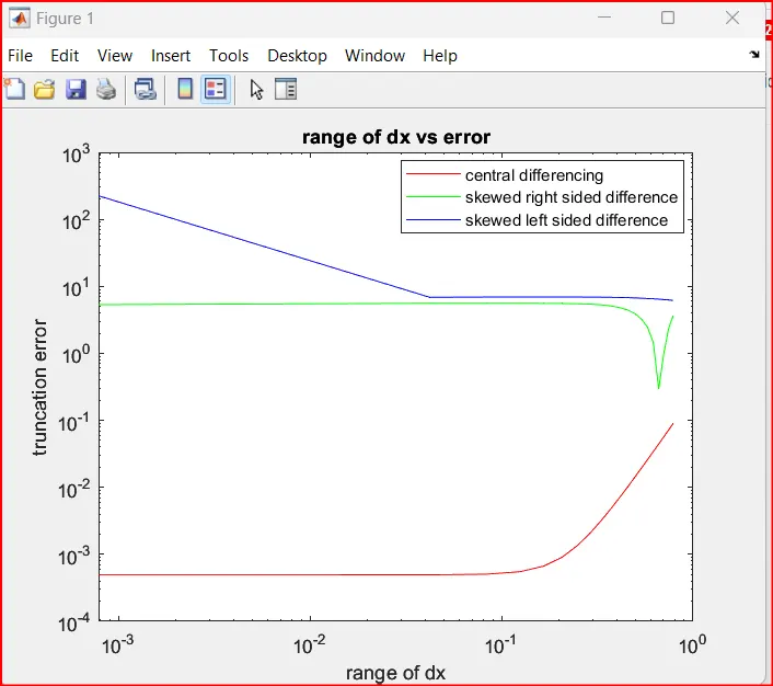
Aim: To Derive the following 4th order approximations of the second-order derivative using Central difference Scheme, Skewed right-sided difference and Skewed left-sided difference using Taylor Table method and compare the obtained results using above schmes with the analytical results for the given function.

Function: `exp(x)*cos(x)`

Number of Nodes:

For central Differencing scheme:

Number of nodes N= p+q-1

p is order of derivative.

q is order of approximations.

no of nodes N = 2+4-1 =5.

For one-sided/skewed schemes:

Number of nodes N= p+q=2+4=6

N=6.

Calculations:

To write the Taylor table:

For Central differencing scheme:

`(del^2u)/(delx^2)=(a f ( i − 2 ) + b f ( i − 1 ) + c f ( i ) + d f ( i + 1 ) + e f ( i + 2 ))/dx^2`

Using taylor series expansion we can compute af(i-2):

`af(i-2)=af(i)-(2af'(i)dx)/(1!)+(4af''(i)dx)/(2!)-(8af'''(i)dx)/(3!)+(16af''''(i)dx)/(4!)`

`nbsp; f(i) f '(i) dx f ''(i) dx^2 f '''(i) dx^3 f ''''(i) dx^4 `

a f(i-2) a -2a 2a `-(4a)/3` `(2a)/3`

b f(i-1) b -b `b/2` `-(b)/6` `b/24`

c f(i) c 0 0 0 0

`f(i+1) d d `d/2` `d/6` `d/24`

e f(i+2) e 2e 2e `(4e)/3` `(2e)/3`

Sum of coefficients 0 0 1 0 0

Since we are finding second order derivative hence the sum of coeffients is 1 for the second order term and remaining all corresponds to zero.

Now writing the coefficients in the matrix form AX=B

`[ [1,-2,2,-4/3,2/3],[1,-1,1/2,-1/6,1/24],[1,0,0,0,0],[1,1,1/2,1/6,1/24],[1,2,2,4/3,2/3] ]*[[a],[b],[c],[d],[e],[g]]=[[0],[0],[1],[0],[0],[0]]`

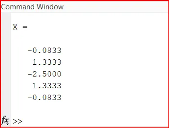
a=-0.0833, b=1.33, c=-2.5, d=1.33, e=-0.0833

``(del^2u)/(delx^2)=((-0.0833) f ( i − 2 ) + (1.33) f ( i − 1 ) + (-2.5) f ( i ) + 1.33 f ( i + 1 ) + (-0.0833) f ( i + 2 ))/dx^2``

Right-sided/skewed schemes:

`(del^2u)/(delx^2)=(a f ( i ) + b f ( i + 1 ) + c f ( i+2 ) + d f ( i + 3 ) + e f ( i + 4 ) + g f ( i + 5 ))/dx^2`

`nbsp; f(i) f '(i) dx f ''(i) dx^2 f '''(i) dx^3 f ''''(i) dx^4 f'''''dx^5`

a f ( i ) a 0 0 0 0 0

b f ( i + 1) b `b` `b/2` `b/6` `b/24` `b/120`

c f ( i + 2) c 2c 2c `(4c)/3` `(2c)/3` `(4c)/5` `

d f ( i + 3) d 3d `(9d)/2` `(9d)/2` `(27d)/8` `(81d)/40`

e f ( i + 4) e 4e 8e `(32e)/3` `(32e)/3` `(128e)/15`

g f ( i + 5) g 5g `(25e)/4` `(125e)/6` `(625e)/24` `(625e)/24`

Sum of 0 0 1 0 0 0

coefficients

Now writing the coefficients in the matrix form AX=B

`[[1,0,0,0,0,0],[1,1,1/2,1/6,1/24,1/120],[1,2,2,4/3,2/3,4/5],[1,3,9/2,9/2,27/8,81/40],[1,4,8,32/3,32/3,128/15],[1,5,25/4,125/6,625/24,625/24]]*[[a],[b],[c],[d],[e],[g]]=[[0],[0],[1],[0],[0],[0]]`

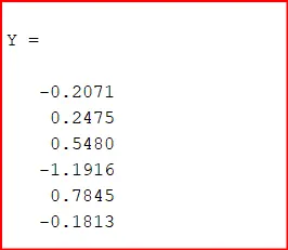
a=-0.2071 , b=0.2475 , c=0.5480, d=-1.1916, e=0.7845 , g=-0.1813

``(del^2u)/(delx^2)=((-0.2071) f ( i ) + (0.2475) f ( i + 1 ) + (0.5480) f ( i+2 ) + (-1.1916) f ( i + 3 ) + (0.7845) f ( i + 4 ) + (-0.1813) f ( i + 5 ))/dx^2``

Left-sided/skewed schemes

`(del^2u)/(delx^2)=(a f ( i -5) + b f ( i - 4 ) + c f ( i - 3) + d f ( i - 2 ) + e f ( i - 1 ) + g f ( i ))/dx^2`

`nbsp; f(i) f '(i) dx f ''(i) dx^2 f '''(i) dx^3 f ''''(i) dx^4 f'''''dx^5`

a f ( i - 5) a -5a `(25a)/4` `-(125a)/6` `(625a)/24` `-(625a)/24`

b f ( i - 4) b -4b 8b `-(32b)/3` `(32b)/3` `-(128b)/15`

c f ( i - 3) c -3c `(9c)/2` `-(9c)/2` `(27c)/8` `(81c)/40`

d f ( i - 2) d -2d 2d `-(4d)/3` `(2d)/3` `-(4d)/5`

e f ( i - 1) e `-e` `e/2` `-e/6` `e/24` `-e/120`

g f ( i ) g 0 0 0 0 0

Sum of 0 0 1 0 0 0

coefficient

Now writing the coefficients in the matrix form AX=B

`[[1,-5,25/4,-125/6,625/24,-625/24],[1,-4,8,-32/3,32/3,-128/15],[1,-3,9/2,-9/2,27/8,81/40],[1,-2,2,-4/3,2/3,-4/5],[1,-1,1/2,-1/6,1/24,-1/120],[1,0,0,0,0,0] ]*[[a],[b],[c],[d],[e],[g]]=[[0],[0],[1],[0],[0],[0]]`

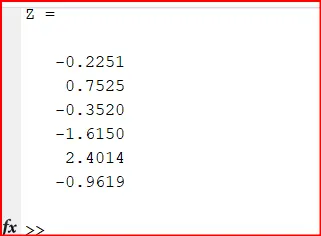
a=-0.2251 , b=0.7525 , c=-0.3520, d=-1.6150, e=2.4014 , g=-0.9619

Substituting the values of coefficient in the above equation

`(del^2u)/(delx^2)=((-0.2251) f ( i -5) + (0.7525) f ( i - 4 ) + (-0.3520) f ( i - 3) + (-1.6150) f ( i - 2 ) + (2.4014) f ( i - 1 ) + (-0.9619) f ( i ))/dx^2`

Matlab Code:

Code to calculate the coefficient of the above matrices

clear all
close all
clc

A=[1,-2,2,-4/3,2/3;1,-1,1/2,-1/6,1/24;1,0,0,0,0;1,1,1/2,1/6,1/24;1,2,2,4/3,2/3];



B=[0;0;1;0;0];

C=[0;0;1;0;0;0];


X=inv(A')*B

R=[1,0,0,0,0,0 ; 1,1,1/2,1/6,1/24,1/120 ; 1,2,2,4/3,2/3,4/5 ; 1,3,9/2,9/2,27/8,81/40 ; 1,4,8,32/3,32/3,128/15 ; 1,5,25/4,125/6,625/24,625/24];

Y=inv(R')*C

L=[1,-5,25/4,-125/6,625/24,-625/24 ; 1,-4,8,-32/3,32/3,-128/15 ; 1,-3,9/2,-9/2,27/8,81/40 ; 1,-2,2,-4/3,2/3,-4/5 ; 1,-1,1/2,-1/6,1/24,-1/120 ; 1,0,0,0,0,0] ;

Z=inv(L')*C

Main Code

clear all
close all
clc

%value of x
x= pi/3;

%range of dx
dx= linspace(pi/4,pi/4000,20);

%for loop
for i=1:length(dx)
    
    central_differencing(i) = fourth_order_central_differencing(x,dx(i));
    
    right_sided_skew(i) = fourth_order_right_sided_skew(x,dx(i));
    
    left_sided_skew(i) = fourth_order_left_sided_skew(x,dx(i));
    
end

%plotting
figure(1)
loglog(dx,central_differencing,'r')
hold on
loglog(dx,right_sided_skew,'g')
hold on
loglog(dx,left_sided_skew,'b')
xlabel('range of dx')
ylabel('truncation error')
title('range of dx vs error')
legend('central differencing','skewed right sided difference','skewed left sided difference','location','northwest')

Function Code

fourth_order_central_differencing

function Error_central_differencing = fourth_order_central_differencing(x,dx)

% analytic function = exp(x)*cos(x)

% analytic derivative
%f''(x) = -2*exp(x)*sin(x)

analytical_derivative = -2*exp(x)*sin(x);

%numerical derivative

%central differencing
central_differencing = (((-0.0833)*((exp(x-(2*dx)))*(cos(x-(2*dx)))))+((1.3333)*((exp(x-dx))*(cos(x-dx))))-((2.5000)*((exp(x))*(cos(x))))+((1.3333)*((exp(x+dx))*(cos(x+dx))))-((0.0833)*((exp(x+(2*dx)))*(cos(x+(2*dx))))))/(dx^2);

%error
Error_central_differencing = abs(central_differencing- analytical_derivative);
end

fourth_order_right_sided_skew

function Error_right_sided_skew = fourth_order_right_sided_skew(x,dx)

% analytic function = exp(x)*cos(x)

% analytic derivative
%f''(x) = -2*exp(x)*sin(x)

analytical_derivative = -2*exp(x)*sin(x);

%numerical derivative


right_sided_skew = (((-0.2071)*((exp(x))*(cos(x))))+((0.2475 )*((exp(x+dx))*(cos(x+dx))))+((0.5480)*((exp(x+(2*dx)))*(cos(x+(2*dx)))))-((1.1916)*((exp(x+(3*dx)))*(cos(x+(3*dx)))))+((0.7845)*((exp(x+(4*dx)))*(cos(x+(4*dx)))))-((0.1813)*((exp(x+(5*dx)))*(cos(x+(5*dx))))))/(dx^2);

%error
Error_right_sided_skew = abs(right_sided_skew- analytical_derivative);
end

function Error_left_sided_skew = fourth_order_left_sided_skew(x,dx)

% analytic function = exp(x)*cos(x)

% analytic derivative
%f''(x) = -2*exp(x)*sin(x)

analytical_derivative = -2*exp(x)*sin(x);

%numerical derivative

left_sided_skew = (((-0.2251)*((exp(x-(5*dx)))*(cos(x-(5*dx)))))+((0.7525 )*((exp(x-(4*dx)))*(cos(x-(4*dx)))))-((0.3520)*((exp(x-(3*dx)))*(cos(x-(3*dx)))))-((1.6150)*((exp(x-(2*dx)))*(cos(x-(2*dx)))))+((2.4014)*((exp(x-dx))*(cos(x-dx))))-((0.9619)*((exp(x))*(cos(x)))))/(dx^2);

%error
Error_left_sided_skew = abs(left_sided_skew- analytical_derivative);
end

Results and plots: