Week 3.5 - Deriving 4th order approximation of a 2nd order derivative using Taylor Table method
Fourth order approximation of a second order derivative:-
1) Central Difference Scheme (CD):-
To find the fourth order numerical approximation of a second order usi
clear all
close all
clc

x = pi/6;                                 %derivative at 30 degree angle
dx = linspace(pi/4,pi/40000,40);
func = exp(x)*cos(x);                     %Function
fdd_A = -2*exp(x)*sin(x);                 %Analytic derivative


a_CD = -0.0833;                           % CD = central Difference
b_CD = 1.3333;
c_CD = -2.5000;
d_CD = 1.3333;
e_CD = -0.0833;

a_RS = 3.7500;                            % RS = Right Skewed
b_RS = -12.8333;
c_RS = 17.8333;
d_RS = -13.0000;
e_RS = 5.0833;
f_RS = -0.8333;

a_LS = -0.8333;                           % LS = Left Skewed
b_LS = 5.0833;
c_LS = -13.0000;
d_LS = 17.8333;
e_LS = -12.8333;
f_LS = 3.7500;

for i = 1:40

    fdd_CD = a_CD*(-2*exp(x-2*dx(i))*sin(x-2*dx(i))) + b_CD*(-2*exp(x-dx(i))*sin(x-dx(i))) + c_CD*(-2*exp(x)*sin(x)) + d_CD *(-2*exp(x+dx(i))*sin(x+dx(i))) + e_CD*(-2*exp(x+2*dx(i))*sin(x+2*dx(i)));
    error_CD(i) = abs(fdd_CD - fdd_A);
    fdd_RS = a_RS*(-2*exp(x)*sin(x)) + b_RS*(-2*exp(x+dx(i))*sin(x+dx(i))) + c_RS*(-2*exp(x+2*dx(i))*sin(x+2*dx(i))) + d_RS*(-2*exp(x+3*dx(i))*sin(x+3*dx(i))) + e_RS*(-2*exp(x+4*dx(i))*sin(x+4*dx(i))) + f_RS*(-2*exp(x+5*dx(i))*sin(x+5*dx(i)));
    error_RS(i) = abs(fdd_RS - fdd_A);
    fdd_LS = a_LS*(-2*exp(x-5*dx(i))*sin(x-5*dx(i))) + b_LS*(-2*exp(x-4*dx(i))*sin(x-4*dx(i))) + c_LS*(-2*exp(x-3*dx(i))*sin(x-3*dx(i))) + d_LS*(-2*exp(x-2*dx(i))*sin(x-2*dx(i))) + e_LS*(-2*exp(x-dx(i))*sin(x-dx(i))) + f_LS*(-2*exp(x)*sin(x));
    error_LS(i) = abs(fdd_LS - fdd_A);
end

plot(dx, error_CD);
hold on;
plot(dx, error_RS);
hold on;
plot(dx, error_LS);
hold off;
xlabel('dx');
ylabel('Error');
legend('Error in Central Difference', 'Error in Right Skewed','Error in Left Skewed');
ng central difference scheme at any point (i) we required 4 points at (i-2), (i-1), (i+1), (i+2) location. As shown in given numerical stencil.
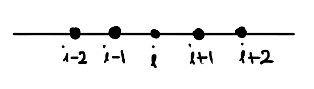
The second order derivative under this scheme is as follows:
`(del^2 f) / (del x^2) = a f_(i-2) + bf_(i-1) + cf_(i) + df_(i+1) + ef_(i+2)` -------eq`
where f = function
and f_i , f_(i-1), f_(i-2), f_(i+1), f_(i+2)
are function values at different points which can be expressed using taylors series expansion at each point.
The Taylors table for this scheme is as follows:
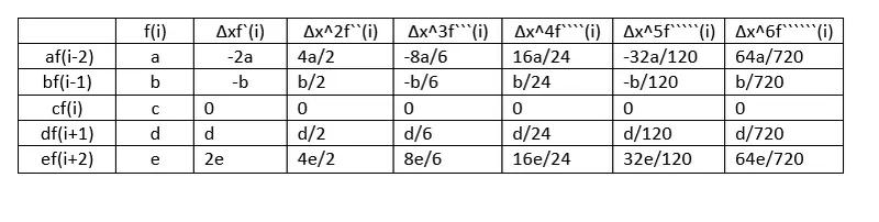
Since the LHS represents the second order derivative then the summation of coefficients of second order derivative in the taylors table is 1 and other will be 0 till 4 as we have assumed only 4 points for approximation in taylor series.
Therefore
a + b + c + d +e = 0
-2a - b + 0 +d + 2e = 0
4a/2 + b/2 + 0 + d/2 + 4e/2 = 1
-8a/6 - b/6 + 0 + d/6 + 8e/6 = 0
16a/24 + b/24 +0 + d/24 + 16e/24 = 0
By solving these equations in matlab we get:-
a = -0.0817
b = 1.3267
c = -2.5
d = 1.3267
e = -0.0817
we can put these values back in equation 1 to check if it is a fourth order approximation or not -
a f_(i-2) + bf_(i-1) + cf_(i) + df_(i+1) + ef_(i+2) = `(Delta x) ^2 fprimeprime(i) + (-32a/120 - b/120 + d/120 + 32e/120) (Deltax)^5 fprimeprimeprimeprimeprime(i) + (64a/720 + b/720 + d/720 + 64e/720)(Deltax)^6 fprimeprimeprimeprimeprimeprime(i)`
= `(Deltax )^2 fprimeprime(i) + (64a/720 + b/720 + d/720 + 64e/720 )Deltax^6 fprimeprimeprimeprimeprimeprime(i)`
by dividing the equation by `(Deltax)^2`
`(del^2 f) / (del x^2) = fprimeprime(i) + ()(Deltax)^4fprimeprimeprimeprimeprimeprime`
Here the last term is neglected to make is a approx second order derivative. The power of differential is 4 of the neglected term .
Hence it is a fourth order approximation.
2) Right Skewed Scheme :- To find the fourth order numerical approximation of a second order using right skewed scheme at any point (i) we required 5 points at (i+1), (i+2), (i+3), (i+4), (i+5) location. As shown in given numerical stencil.
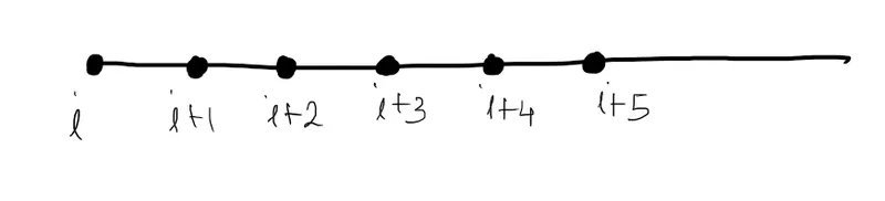
The second order derivative under this scheme is as follows:
`(del^2 f) / (del x^2) = a f_(i) + bf_(i+1) + cf_(i+2) + df_(i+3) + ef_(i+4) + g_(i+5)` -------eq 2`
where f = function
`nd f_i , f_(i+1), f_(i+2), f_(i+3), f_(i+4), f_(i+5)`
are function values at different points which can be expressed using taylors series expansion at each point.
The Taylors table for this scheme is as follows:
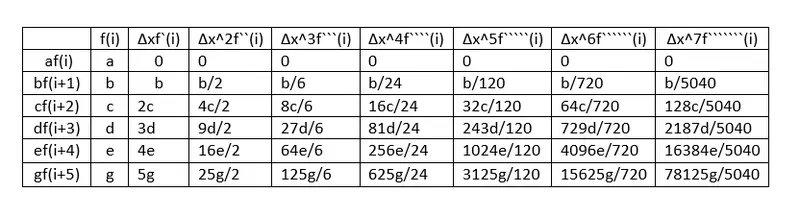
Since the LHS represents the second order derivative then the summation of coefficients of second order derivative in the taylors table is 1 and other will be 0 till 5 as we have assumed only 5 points for approximation in taylor series.
Therefore
a + b + c + d + e + g = 0
b + 2c + 3d + 4e + 5g = 0
b/2 + 4c/2 + 9d/2 + 16e/2 + 25g/2 = 1
b/6 + 8c/6 + 27d/6 + 64e/6 + 125g/6 = 0
b/24 +16c/24 + 81d/24 + 256e/24 + 625g/24 = 0
b/120 + 32c/120 + 243d/120 + 1024e/120 + 3125g/120 = 0
By solving these equations in matlab we get:-
a = -25.5815
b = 124.0103
c = -236.2436
d = 221.4839
e = -102.3706
g = 18.7016
we can put these values back in equation 1 to check if it is a fourth order approximation or not -
`a f_(i) + bf_(i+1) + cf_(i+2) + df_(i+3) + ef_(i+4) + g_(i+5) = (Deltax)^2fprimeprime(i) + (b/720 + 64c/720 + 729d/720 + 4096e/720 + 15625g/720) (Deltax)^6 fprimeprimeprimeprimeprimeprime(i) + ( b/5040 + 128c/5040 + 218d/5040 + 16384e/5040 + 78125g/5040)(Deltax)^7fprimeprimeprimeprimeprimeprimeprime(i)`
`a f_(i) + bf_(i+1) + cf_(i+2) + df_(i+3) + ef_(i+4) + g_(i+5) = (Deltax)^2fprimeprime(i) + (2600) (Deltax)^6 fprimeprimeprimeprimeprimeprime(i) + (1100)(Deltax)^7fprimeprimeprimeprimeprimeprimeprime(i)`
dividing the equation by (`Delta x`)^2 to get the approx second derivative we get
`(del^2 f) / (del x^2) = fprimeprime(i) + 2600(Deltax)^4fprimeprimeprimeprimeprimeprime(i) + 1100(Deltax)^5fprimeprimeprimeprimeprimeprimeprime(i)`
To get the approx second order derivative term the highest order neglected is 4.
Hence it is a fourth order approximation.
3) Left Skewed Scheme:- `o find the fourth order numerical approximation of a second order using right skewed scheme at any point (i) we required 5 points at (i-1), (i-2), (i-3), (i-4), (i-5) location. As shown in given numerical stencil`
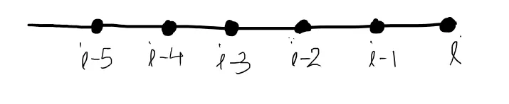
The second order derivative under this scheme is as follows:
`(del^2 f) / (del x^2) = a f_(i-5) + bf_(i-4) + cf_(i-3) + df_(i-2) + ef_(i-1) + g_(i)` -------eq 3`
where f = function
`nd f_i , f_(i-1), f_(i-2), f_(i-3), f_(i-4), f_(i-5)`
are function values at different points which can be expressed using taylors series expansion at each point.
The Taylors table for this scheme is as follows:
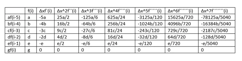
Since the LHS represents the second order derivative then the summation of coefficients of second order derivative in the taylors table is 1 and other will be 0 till 5 as we have assumed only 5 points for approximation in taylor series.
Therefore
a + b + c + d + e + g = 0
-5a -4b -3c -2d -e + 0 = 0
25a/2 + 16b/2 + 9d/2 + 4e/2 + e/2 + 0 = 1
-125a/6 -64b/6 -27c/6 -8d/6 -e/6 + 0 = 0
625a/24 + 256b/24 + 81c/24 + 16d/24 + e/24 + 0 = 0
-3125a/120 -1024b/120 -243c/120 -32d/120-e/120 = 0
By solving these equations in matlab we get:-
a = -0.8456
b = 5.1458
c = -13.1188
d = 17.9374
e = -12.8738
g = 3.7549
we can put these values back in equation 3 to check if it is a fourth order approximation or not -
`af_(i-5) + bf_(i-4) + cf_(i-3) + df_(i-2) + ef_(i-1) + g = (Deltax)^2fprimeprime(i) + (15625a/720 + 4096b/720 +729c/720 +64d/720 +e/720)(Deltax)^6fprimeprimeprimeprimeprimeprime(i) + (-78125a/5040 -16384b/5040 -2187c/5040 -128d/5040 -e/5040)(Deltax)^7fprimeprimeprimeprimeprimeprimeprime(i)`
dividing the equation by (`Delta x`)^2 to get the approx second derivative we get
`af_(i-5) + bf_(i-4) + cf_(i-3) + df_(i-2) + ef_(i-1) + g = fprimeprime(i) + (15625a/720 + 4096b/720 +729c/720 +64d/720 +e/720)(Deltax)^4fprimeprimeprimeprimeprimeprime(i) + (-78125a/5040 -16384b/5040 -2187c/5040 -128d/5040 -e/5040)(Deltax)^5fprimeprimeprimeprimeprimeprimeprime(i)`
To get the approx second order derivative term the highest order neglected is 4.
Hence it is a fourth order approximation.
A skewed scheme can be benificial over central or symmetric scheme for computing values at the boundaries. Because the values at left hand side or right hand side of the boundaries are not known so a central scheme cannot be used there for computaional purposes. Therefore skewed schemes are important there.