Week 3.5 - Deriving 4th order approximation of a 2nd order derivative using Taylor Table method
Objective:
Deriving 4th order approximations of the second-order derivative
1. Central difference
Number of nodes =P+Q-1 (for all central difference schemes)
where; P=order of derivatives
Q=order of approximation
In this problem our requirement is second order derivatives and Fourth order approximation
so P=2, Q=4
No. OF nodes=5
Hypothesis equation
`f(u,x)=(partial^2 u)/(partialx^2)=a.f(i-2)+b.f(i-1)+c.f(i)+d.f(i+1)+e.f(i+2)`
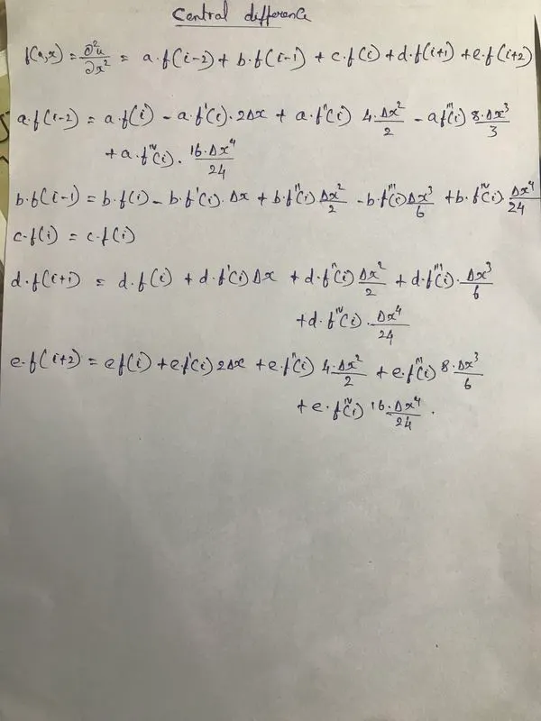
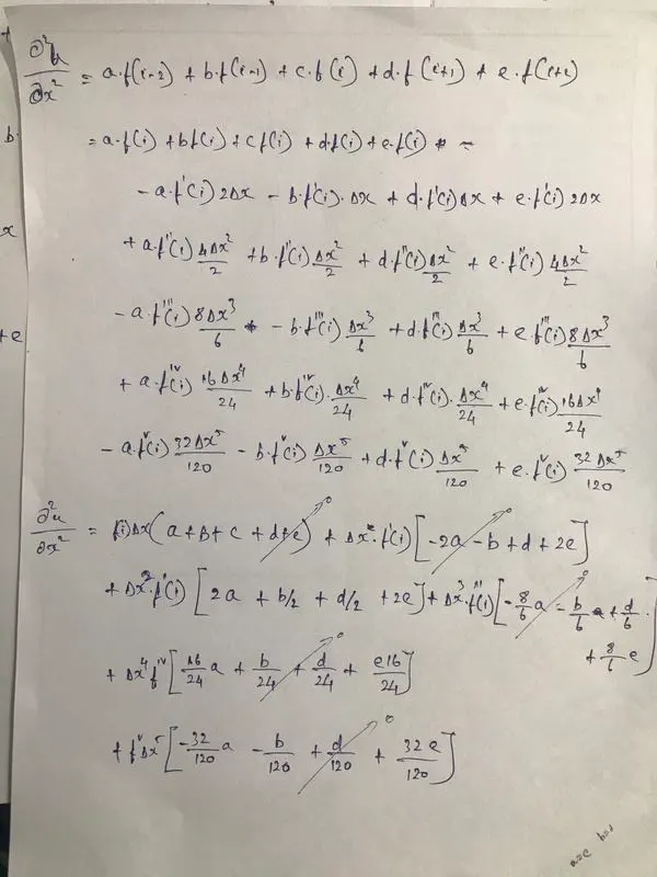
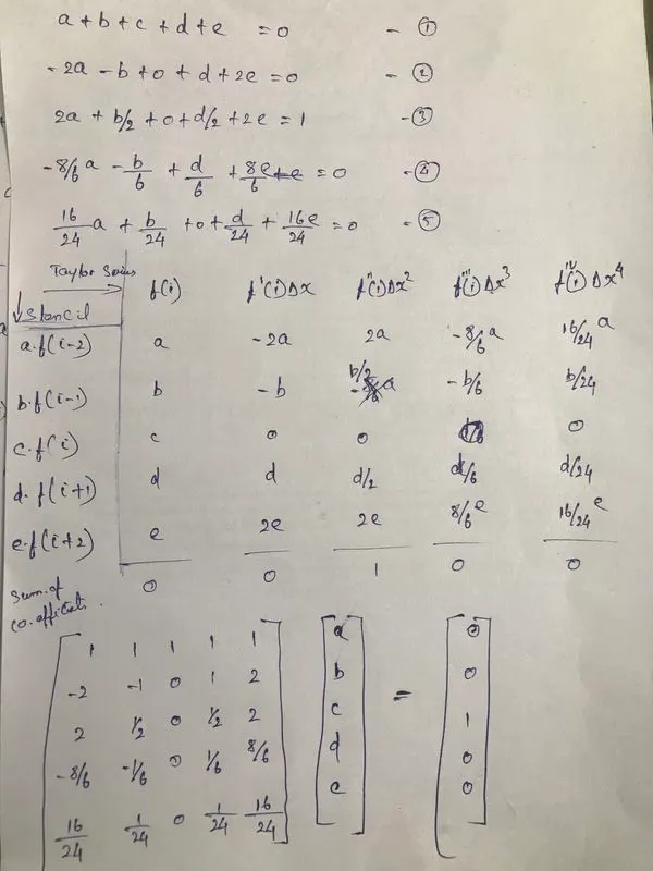
>> A=[1 1 1 1 1;-2 -1 0 1 2;2 1/2 0 1/2 2;-8/6 -1/6 0 1/6 8/6;16/24 1/24 0 1/24 16/24]

A =

    1.0000    1.0000    1.0000    1.0000    1.0000
   -2.0000   -1.0000         0    1.0000    2.0000
    2.0000    0.5000         0    0.5000    2.0000
   -1.3333   -0.1667         0    0.1667    1.3333
    0.6667    0.0417         0    0.0417    0.6667

>> B=[0;0;1;0;0]

B =

     0
     0
     1
     0
     0

>> X=inv(A)*B

X =

   -0.0833
    1.3333
   -2.5000
    1.3333
   -0.0833

>>
a=-0.0833, b=1.3333, c=-2.50, d=1.3333, e=-0.0833
`f(u,x)=(partial^2 u)/(partialx^2)=(a.f(i-2)+b.f(i-1)+c.f(i)+d.f(i+1)+e.f(i+2))/(Delta x^2)`
Central difference
`(partial^2 u)/(partialx^2)=(-0.0833.f(i-2)+1.3333.f(i-1)-2.5.f(i)+1.3333.f(i+1)-0.0833.f(i+2))/(Delta x^2)`
2. Skewed right-sided difference
Number of nodes =P+Q (for all skewed schemes)
where; P=order of derivatives
Q=order of approximation
In this problem our requirement is second order derivatives and Fourth order approximation
so P=2, Q=4
No. OF nodes=6
Hypothesis equation
`f(u,x)=(partial^2 u)/(partialx^2)=a.f(i)+b.f(i+1)+c.f(i+2)+d.f(i+3)+e.f(i+4)+g.f(i+5)`
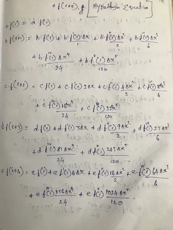
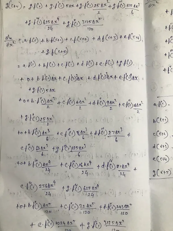
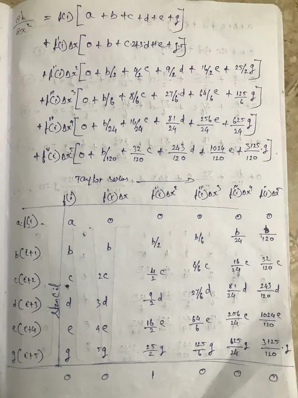
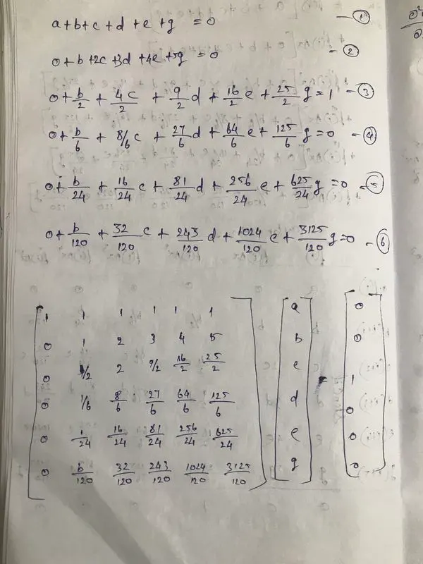
>> A=[1 1 1 1 1 1;0 1 2 3 4 5;0 1/2 4/2 9/2 16/2 25/2;0 1/6 8/6 27/6 64/6 125/6;0 1/24 16/24 81/24 256/24 625/24;0 1/120 32/120 243/120 1024/120 3125/120]

A =

    1.0000    1.0000    1.0000    1.0000    1.0000    1.0000
         0    1.0000    2.0000    3.0000    4.0000    5.0000
         0    0.5000    2.0000    4.5000    8.0000   12.5000
         0    0.1667    1.3333    4.5000   10.6667   20.8333
         0    0.0417    0.6667    3.3750   10.6667   26.0417
         0    0.0083    0.2667    2.0250    8.5333   26.0417

>> B=[0;0;1;0;0;0]

B =

     0
     0
     1
     0
     0
     0

>> X=inv(A)*B

X =

    3.7500
  -12.8333
   17.8333
  -13.0000
    5.0833
   -0.8333

>>
a=3.7500, b=-12.8333, c=17.8333, d=-13, e=5.0833, g=-0.8333.
`f(u,x)=(partial^2 u)/(partialx^2)=(a.f(i)+b.f(i+1)+c.f(i+2)+d.f(i+3)+e.f(i+4)+g.f(i+5))/(Delta x^2)`
Fourth order approximation of second order derivative by skewed right sided difference
`f(u,x)=(partial^2 u)/(partialx^2)=(3.7500*f(i)-12.8333*f(i+1)+17.8333.f(i+2)-13*.f(i+3)+5.0833.f(i+4)-0.8333.f(i+5))/(Delta x^2)`
3. Skewed left-sided difference
Number of nodes =P+Q=>2+4=6.
Hypothesis equation
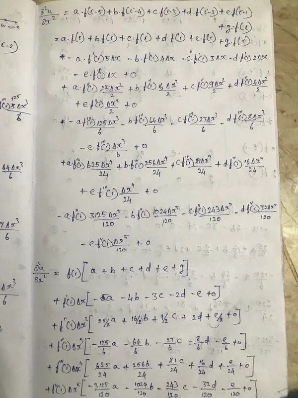
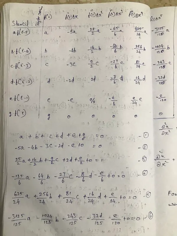
`f(u,x)=(partial^2 u)/(partialx^2)=a.f(i-5)+b.f(i-4)+c.f(i-3)+d.f(i-2)+e.f(i-1)+g.f(i)`
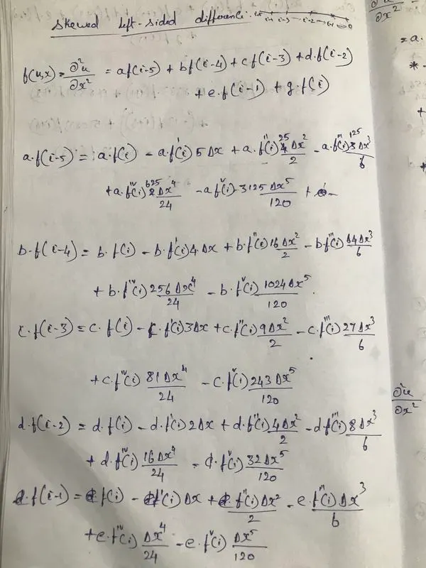
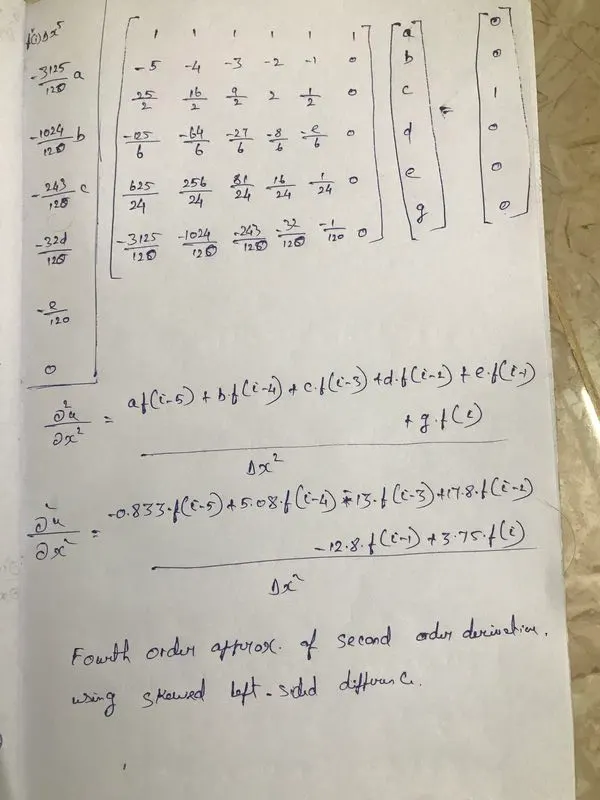
>> A=[1 1 1 1 1 1;-5 -4 -3 -2 -1 0;25/2 16/2 9/2 2 1/2 0;-125/6 -64/6 -27/6 -8/6 -1/6 0;625/24 256/24 81/24 16/24 1/24 0;-3125/120 -1024/120 -243/120 -32/120 -1/120 0]

A =

    1.0000    1.0000    1.0000    1.0000    1.0000    1.0000
   -5.0000   -4.0000   -3.0000   -2.0000   -1.0000         0
   12.5000    8.0000    4.5000    2.0000    0.5000         0
  -20.8333  -10.6667   -4.5000   -1.3333   -0.1667         0
   26.0417   10.6667    3.3750    0.6667    0.0417         0
  -26.0417   -8.5333   -2.0250   -0.2667   -0.0083         0

>> B=[0;0;1;0;0;0]

B =

     0
     0
     1
     0
     0
     0

>> X=inv(A)*B

X =

   -0.8333
    5.0833
  -13.0000
   17.8333
  -12.8333
    3.7500

>>
a=-0.8333, b=5.0833, c=-13, d=17.8333, e=-12.8333, g=3.7500
`(partial^2 u)/(partialx^2)=(a.f(i-5)+b.f(i-4)+c.f(i-3)+d.f(i-2)+e.f(i-1)+g.f(i))/(Delta x^2)`
Fourth order approximation of second order derivative by skewed left sided difference
`(partial^2 u)/(partialx^2)=(-0.8333.f(i-5)+5.0833.f(i-4)-13.f(i-3)+17.8333.f(i-2)-12.8333.f(i-1)+3.7500.f(i))/(Delta x^2)`
Function program for central difference scheme
function [cd_error]=central_difference(x,dx)


%analytical function = exp(x)*cos(x)
exact_derivative =-2*exp(x)*sin(x)

%numerical derivative
central_difference=(((-0.0833*exp(x-(2*dx))*cos(x-(2*dx)))+(1.3333*exp(x-dx)*cos(x-dx))-(2.5000*exp(x)*cos(x))+(1.3333*exp(x+dx)*cos(x+dx))-(0.0833*exp(x+(2*dx))*cos(x+(2*dx)))))/(dx)^2


%Error
cd_error=abs(central_difference-exact_derivative)

end
Function program for right sided skewed scheme
function [error_skewed_right]=right_skewed_difference(x,dx)

%analytical function = exp(x)*cos(x)
exact_derivative =-2*exp(x)*sin(x)

%numerical derivative
right_skewed_difference=((3.7500*exp(x)*cos(x))-(12.8333*exp(x+dx)*cos(x+dx))+(17.8333*exp(x+(2*dx))*cos(x+(2*dx)))-(13*exp(x+(3*dx))*cos(x+(3*dx)))+(5.0833*exp(x+(4*dx))*cos((x+4*dx)))-(0.8333*exp(x+(5*dx))*cos(x+(5*dx))))/(dx)^2


%Error
[error_skewed_right]=abs(right_skewed_difference-exact_derivative)

end
Function program for left sided skewed scheme
function [error_lsd]=left_skewed_difference(x,dx)

%analytical function = exp(x)*cos(x)
exact_derivative =-2*exp(x)*sin(x)

%numerical derivative
left_skewed_difference=(((-0.8333*exp(x-(5*dx))*cos(x-(5*dx))+5.0833*exp(x-(4*dx))*cos(x-(4*dx))-13*exp(x-(3*dx))*cos(x-(3*dx))+17.8333*exp(x-(2*dx))*cos(x-(2*dx))-12.8333*exp(x-dx)*cos(x-dx))+3.7500*exp(x)*cos(x)))/(dx)^2


%Error
[error_lsd]=abs(left_skewed_difference-exact_derivative)

end
Main program
clear all
close all
clc

x=pi/3;
dx= linspace(pi/40,pi/4000,20)


for i=1:length(dx)

    error_cd(i)=central_difference(x,dx(i))
    error_right_skewed(i)=right_skewed_difference(x,dx(i))
    error_left_skewed(i)=left_skewed_difference(x,dx(i))

end


%Plotting

loglog(dx,error_cd,'LineWidth',1,'Marker','*')
hold on
loglog(dx,error_right_skewed,'LineWidth',1,'Marker','*')
hold on
loglog(dx,error_left_skewed,'LineWidth',1,'Marker','*')
xlabel('dx')
ylabel('errors')
legend('central difference','right side skewed','left side skewed')
Output:
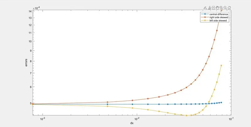
As we can see, comparing other two schemes central difference scheme is more accurate and it takes the information from both sides to give that accurate values.
why a skewed scheme is useful?
If we want to compute from one end where the central scheme cant comes to play, we can use skewed scheme.
What can a skewed scheme do that a CD scheme cannot?
In central difference we need node balance from both side, in skewed scheme we dont need that.