Week 3.5 - Deriving 4th order approximation of a 2nd order derivative using Taylor Table method
AIM
- Derive the 4th order approximations of the second-order derivative for
- Central difference
- Skewed right-sided difference
- Skewed left-sided difference
- Prove the skewed scheme are fourth order accurate
- Write a program to evaluate second-order derivative of the analytical function `e^x*cosx` and compare it with the 3 numerical approximations that you have derived
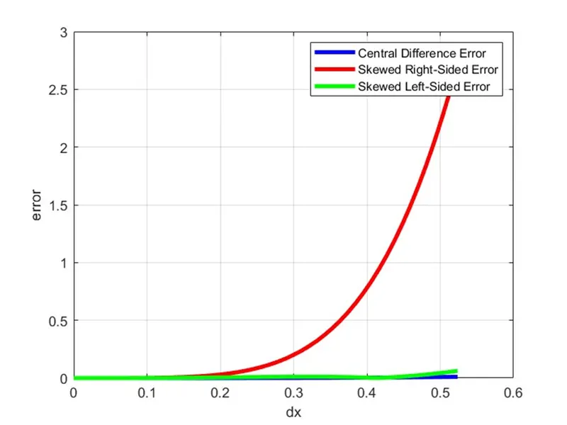
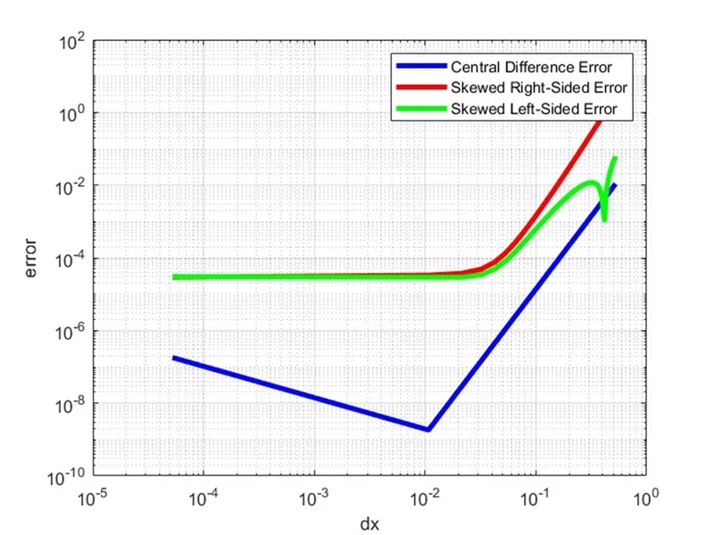
- Plot a graph comparing the errors between each of the schemes
- Describe use of Skewed scheme and its advantage over Central Difference Scheme
GOVERNING EQUATIONS
- Fourth Order Approximation of second-order Derivative using Central Differencing Scheme

- Numerical Stencil for the Central difference Scheme is as shown above where `i` represents the node under investigation where 4th order Approximation is computed and `(i-2)`, `(i-1)`, `(i+1)`, `(i+2)` represents the closest node from which the key information required for the approximation are gathered. These nodes are `Deltax` apart for each other
- So, based on the above information the hypothesis equation for second order derivative using Central Difference Scheme will be `(del^2u)/(delx^2) = af(i-2)+bf(i-1)+cf(i)+df(i+1)+ef(i+2)` where value of `a,b,c,d,e` are derived by solving using Tayler Table method
- Fourth Order Approximation of second-order Derivative using Skewed Right-Side Difference Scheme

- Numerical Stencil for the Skewed Right-Side difference Scheme is as shown above where `i` represents the node under investigation where 4th order Approximation is computed and `(i+1)`, `(i+2)`, `(i+3)`, `(i+4)` and `(i+5)` represents the closest node to the right from which the key information required for the approximation are gathered. These nodes are `Deltax` apart for each other
- So, based on the above information the hypothesis equation for second order derivative using Central Difference Scheme will be `(del^2u)/(delx^2) = af(i)+bf(i+1)+cf(i+2)+df(i+3)+ef(i+4)+gf(i+5)` where value of `a,b,c,d,e,g` are derived by solving using Tayler Table method
- Fourth Order Approximation of second-order Derivative using Skewed Left-Side Differencing Scheme

- Numerical Stencil for the Skewed Left-Side difference Scheme is as shown above where `i` represents the node under investigation where 4th order Approximation is computed and `(i-5)`, `(i-4)`, `(i-3)`, `(i-2)`, `(i-1)` represents the closest node to the left from which the key information required for the approximation are gathered. These nodes are `Deltax` apart for each other
- So, based on the above information the hypothesis equation for second order derivative using Central Difference Scheme will be `(del^2u)/(delx^2) = af(i-5)+bf(i-4)+cf(i-3)+df(i-2)+ef(i-1)+gf(i)` where value of `a,b,c,d,e,g` are derived by solving using Tayler Table method
OBJECTIVE
- Understand how different Scheme for fourth order Approximation works
- Learn the ease of solving Hypothetical Equation using Taylor Table
- Understand the accuracy of each Difference Scheme and the Practical use of the scheme under different scenarios
BODY
Derivation of 4th Order Approximation of second Order Derivative using Central Difference Method
The Hypothetical Equation for the Second Order Derivative can be given as
`(del^2u)/(delx^2) = af(i-2)+bf(i-1)+cf(i)+df(i+1)+ef(i+2)`
Where `a,b,c,d,e` are derived by solving using Tayler Table method
According to Taylor’s Series,
`a.f(i-2) = a.f(i) - a.((2Deltax)f'(i))/(1!)+a.((2Deltax)^2f''(i))/(2!)-a.((2Deltax)^3f'''(i))/(3!)+a.((2Deltax)^4f''''(i))/(4!)-a.((2Deltax)^5f'''''(i))/(5!)+a.((2Deltax)^6f''''''(i))/(6!)`
`b.f(i-1) = b.f(i) - b.((Deltax)f'(i))/(1!)+b.((Deltax)^2f''(i))/(2!)-b.((Deltax)^3f'''(i))/(3!)+b.((Deltax)^4f''''(i))/(4!)-b.((Deltax)^5f'''''(i))/(5!)+b.((Deltax)^6f''''''(i))/(6!)`
`c.f(i) = c.f(i)`
`d.f(i+1) = d.f(i) + d.((Deltax)f'(i))/(1!)+d.((Deltax)^2f''(i))/(2!)+d.((Deltax)^3f'''(i))/(3!)+d.((Deltax)^4f''''(i))/(4!)+d.((Deltax)^5f'''''(i))/(5!)+d.((Deltax)^6f''''''(i))/(6!)`
`e.f(i+2) = e.f(i) + e.((2Deltax)f'(i))/(1!)+e.((2Deltax)^2f''(i))/(2!)+e.((2Deltax)^3f'''(i))/(3!)+e.((2Deltax)^4f''''(i))/(4!)+e.((2Deltax)^5f'''''(i))/(5!)+e.((2Deltax)^6f''''''(i))/(6!)`
The Above equations can be divided and represented in Table format as below
|
`f(i)` |
`Deltaxf'(i)` |
`Deltax^2f''(i)` |
`Deltax^3f'''(i)` |
`Deltax^4f''''(i)` |
`Deltax^5f'''''(i)` |
`Deltax^6f''''''(i)` |
|
|
`a.f(i-2)` |
`a` |
`-2a` |
`2a` |
`(-4a)/3` |
`(2a)/3` |
`(-4a)/15` |
`(4a)/45` |
|
`b.f(i-1)` |
`b` |
`-b` |
`b/2` |
`(-b)/6` |
`b/24` |
`(-b)/120` |
`b/720` |
|
`c.f(i)` |
`c` |
`0` |
`0` |
`0` |
`0` |
`0` |
`0` |
|
`d.f(i+1)` |
`d` |
`d` |
`d/2` |
`d/6` |
`d/24` |
`d/120` |
`d/720` |
|
`e.f(i+2)` |
`e` |
`2e` |
`2e` |
`(4e)/3` |
`(2e)/3` |
`(4e)/15` |
`(4e)/45` |
|
`(del^2u)/(delx^2)` |
`0` |
`0` |
`1` |
`0` |
`0` |
`?` |
`?` |
Only the first 5 Equations will be used to determine the values of `a,b,c,d,e`. However, when we add like terms that we get after expanding the functions on RHS, we know that sum of coefficient of `f(i)`, `Deltaxf'(i)`, `Deltax^3f'''(i)`, `Deltax^4f''''(i)` equates to Zero as we compare it with LHS. While, Coefficient of `Deltax^2f''(i)` equates to 1. These Equations can be represented in the form of Matrix as below
`a+b+c+d+e=0` - 1
`-2a-b+d+2e=0` - 2
`2a+b/2+d/2+2e=1` - 3
`(-4a)/3+(-b)/6+d/6+(4e)/3=0` -4
`(2a)/3+b/24+d/24+(2e)/3=0` - 5
`[[1,1,1,1,1],[-2,-1,0,1,2],[2,1/2,0,1/2,2],[-4/3,-1/6,0,1/6,4/3],[2/3,1/24,0,1/24,2/3]].[[a],[b],[c],[d],[e]] = [[0],[0],[1],[0],[0]]`
On solving the above matrix, we get
`[[a],[b],[c],[d],[e]]=[[-1/12],[4/3],[-5/2],[4/3],[-1/12]]`
From the above equation we can see that `a=e` and `b=d`
Now, as we divide the `Deltax^2` and substituting all values on the RHS we get,
`(del^2u)/(delx^2) = (af(i-2)+bf(i-1)+cf(i)+df(i+1)+ef(i+2))/( Deltax^2)`
`(del^2u)/(delx^2) = ((-1/12)f(i-2)+(4/3)f(i-1)+(-5/2)f(i)+(4/3)f(i+1)+(-1/12)f(i+2))/( Deltax^2)`
Also, on expanding the hypothetical Equation,
`(del^2u)/(delx^2) = (a+b+c+d+e)f(i)+(-2a-b+0+d+2e)Deltaxf'(i)+(2a+b/2+0+d/2+2e)Deltax^2f''(i)+((-4a)/3+(-b)/6+0+d/6+(4e)/3)Deltax^3f'''(i)+((2a)/3+b/24+0+d/24+(2e)/3)Deltax^4f''''(i)+((-4a)/15+(-b)/120+0+d/120+(4e)/15)Deltax^5f'''''(i)+((4a)/45+b/720+0+d/720+(4e)/45)Deltax^6f''''''(i)`
From the above equation and Substituting values of variables we get
`(del^2u)/(delx^2) = (2a+b/2+0+d/2+2e)Deltax^2f''(i)+ ((4a)/45+b/720+0+d/720+(4e)/45) Deltax^6f''''''(i)`
`(del^2u)/(delx^2) = (2(-1/12)+(4/3)/2+0+(4/3)/2+2(-1/12))Deltax^2f''(i)+ ((4(-1/12))/45+(4/3)/720+0+(4/3)/720+(4(-1/12))/45) Deltax^6f''''''(i)`
On Dividing by `Deltax^2`,
`(del^2u)/(delx^2) = (2a+b/2+0+d/2+2e)f''(i)+ ((4a)/45+b/720+0+d/720+(4e)/45) Deltax^4f''''''(i)`
`(del^2u)/(delx^2) = (2(-1/12)+(4/3)/2+0+(4/3)/2+2(-1/12))f''(i)+ ((4(-1/12))/45+(4/3)/720+0+(4/3)/720+(4(-1/12))/45) Deltax^4f''''''(i)`
In the above equation, the term `Deltax^4`, denotes the truncation error. Here, we can see that the order of the truncation error - `[O(Deltax^4)]` is ‘4’. Since we know that the order of approximation is defined by the truncation error term. Therefore, we can say that our central difference scheme is 4th order accurate.
Derivation of 4th Order Approximation of second Order Derivative using Skewed Right Side Difference Method
For the derivation of second Order Derivative using Skewed Right Side Difference Method, information from 5 closest node to the Right Side is required
The Hypothetical Equation for the Second Order Derivative can be given as
`(del^2u)/(delx^2) = af(i)+bf(i+1)+cf(i+2)+df(i+3)+ef(i+4)+gf(i+5)`
where value of `a,b,c,d,e,g` are derived by solving using Tayler Table method
According to Taylor’s Series,
`a.f(i) = a.f(i)`
`b.f(i+1) = b.f(i) + b.((Deltax)f'(i))/(1!) +b.((Deltax)^2f''(i))/(2!)+ b.((Deltax)^3f'''(i))/(3!)+ b.((Deltax)^4f''''(i))/(4!)+ b.((Deltax)^5f'''''(i))/(5!)+b.((Deltax)^6f''''''(i))/(6!)`
`c.f(i+2) = c.f(i) + c.((2Deltax)f'(i))/(1!)+ c.((2Deltax)^2f''(i))/(2!)+ c.((2Deltax)^3f'''(i))/(3!)+ c.((2Deltax)^4f''''(i))/(4!)+ c.((2Deltax)^5f'''''(i))/(5!)+ c.((2Deltax)^6f''''''(i))/(6!)`
`d.f(i+3) = d.f(i) + d.((3Deltax)f'(i))/(1!)+d.((3Deltax)^2f''(i))/(2!)+d.((3Deltax)^3f'''(i))/(3!)+d.((3Deltax)^4f''''(i))/(4!)+d.((3Deltax)^5f'''''(i))/(5!)+d.((3Deltax)^6f''''''(i))/(6!)`
`e.f(i+4) = e.f(i) + e.((4Deltax)f'(i))/(1!)+e.((4Deltax)^2f''(i))/(2!)+e.((4Deltax)^3f'''(i))/(3!)+e.((4Deltax)^4f''''(i))/(4!)+e.((4Deltax)^5f'''''(i))/(5!)+e.((4Deltax)^6f''''''(i))/(6!)`
`g.f(i+5) = g.f(i) + g.((5Deltax)f'(i))/(1!)+ g.((5Deltax)^2f''(i))/(2!)+ g.((5Deltax)^3f'''(i))/(3!)+ g.((5Deltax)^4f''''(i))/(4!)+ g.((5Deltax)^5f'''''(i))/(5!)+ g.((5Deltax)^6f''''''(i))/(6!)`
The Above equations can be divided and represented in Table format as below
|
`f(i)` |
`Deltaxf'(i)` |
`Deltax^2f''(i)` |
`Deltax^3f'''(i)` |
`Deltax^4f''''(i)` |
`Deltax^5f'''''(i)` |
`Deltax^6f''''''(i)` |
|
|
`a.f(i)` |
`a` |
`0` |
`0` |
`0` |
`0` |
`0` |
`0` |
|
`b.f(i+1)` |
`b` |
`b` |
`b/2` |
`b/6` |
`b/24` |
`b/120` |
`b/720` |
|
`c.f(i+2)` |
`c` |
`2c` |
`2c` |
`(4c)/3` |
`(2c)/3` |
`(4c)/15` |
`(4c)/45` |
|
`d.f(i+3)` |
`d` |
`3d` |
`(9d)/2` |
`(9d)/2` |
`27d/8` |
`81d/40` |
`81d/80` |
|
`e.f(i+4)` |
`e` |
`4e` |
`8e` |
`(32e)/3` |
`(32e)/3` |
`(128e)/15` |
`(256e)/45` |
|
`g.f(i+5)` |
`g` |
`5g` |
`(25g)/2` |
`(125g)/6` |
`(625g)/24` |
`(625g)/24` |
`(3125g)/144` |
|
`(del^2u)/(delx^2)` |
`0` |
`0` |
`1` |
`0` |
`0` |
`0` |
`?` |
Only the first 6 Equations will be used to determine the values of `a,b,c,d,e,g`. However, when we add like terms that we get after expanding the functions on RHS, we know that sum of coefficient of `f(i)`, `Deltaxf'(i)`, `Deltax^3f'''(i)`, `Deltax^4f''''(i)` and `Deltax^5f''''(i)` equates to Zero as we compare it with LHS. While Coefficient of `Deltax^2f''(i)` equates to 1. These Equations can be represented in the form of Matrix as below
`a+b+c+d+e+g=0` - 1
`b+2c+3d+4e+5g=0` - 2
`b/2+2c+(9d)/2+8e+(25g)/2=1` - 3
`b/6+(4c)/3+(9d)/2+(32e)/3+(125g)/6=0` -4
`b/24+(2c)/3+27d/8+(32e)/3+(625g)/24=0` - 5
`b/120+(4c)/15+81d/40+(128e)/15+(625g)/24=0` - 6
`[[1,1,1,1,1,1],[0,1,2,3,4,5],[0,1/2,2,9/2,8,25/2],[0,1/6,4/3,9/2,32/3,125/6],[0,1/24,2/3,27/8,32/3,625/24],[0,1/120,4/15,81/40,128/15,625/24]].[[a],[b],[c],[d],[e],[g]] = [[0],[0],[1],[0],[0],[0]]`
On solving the above matrix, we get
`[[a],[b],[c],[d],[e],[g]]=[[15/4],[-77/6],[107/6],[-13],[61/12],[-5/6]]`
Now, as we divide the `Deltax^2` and substituting all values on the RHS we get,
`(del^2u)/(delx^2) = (af(i)+bf(i+1)+cf(i+2)+df(i+3)+ef(i+4)+gf(i+5))/( Deltax^2)`
`(del^2u)/(delx^2) = ((15/4)f(i)-(77/6)f(i+1)+(107/6)f(i+2)-13f(i+3)+(61/12)f(i+4)-(5/6)f(i+5))/( Deltax^2)`
Also, on expanding the hypothetical Equation,
`(del^2u)/(delx^2) = (a+b+c+d+e+g)f(i)+( b+2c+3d+4e+5g) Deltaxf'(i)+ (b/2+2c+(9d)/2+8e+(25g)/2)Deltax^2f''(i)+ (b/6+(4c)/3+(9d)/2+(32e)/3+(125g)/6)/3)Deltax^3f'''(i)+ (b/24+(2c)/3+27d/8+(32e)/3+(625g)/24)Deltax^4f''''(i)+ (b/120+(4c)/15+81d/40+(128e)/15+(625g)/24)Deltax^5f'''''(i)+ (b/720+(4c)/45+81d/80+(256e)/45+(3125g)/144)Deltax^6f''''''(i)`
From the above equation and Substituting values of variables we get
`(del^2u)/(delx^2) = (b/2+2c+(9d)/2+8e+(25g)/2)Deltax^2f''(i)+ (b/720+(4c)/45+81d/80+(256e)/45+(3125g)/144) Deltax^6f''''''(i)`
`(del^2u)/(delx^2) = ((-77/6)/2+2(107/6)+(9/2)(-13)+8(61/12)+(25/2)(-5/6))Deltax^2f''(i)+ ((-77/6)/720+(4(107/6))/45+(81/80)(-13)+(256/45)(61/12)+(3125/144)(-5/6)) Deltax^6f''''''(i)`
On Dividing by `Deltax^2`,
`(del^2u)/(delx^2) = (b/2+2c+(9d)/2+8e+(25g)/2)f''(i)+ (b/720+(4c)/45+81d/80+(256e)/45+(3125g)/144) Deltax^4f''''''(i)`
`(del^2u)/(delx^2) = ((-77/6)/2+2(107/6)+(9/2)(-13)+8(61/12)+(25/2)(-5/6))f''(i)+ ((-77/6)/720+(4(107/6))/45+(81/80)(-13)+(256/45)(61/12)+(3125/144)(-5/6)) Deltax^4f''''''(i)`
In the above equation, the term `Deltax^4`, denotes the truncation error. Here, we can see that the order of the truncation error - `[O(Deltax^4)]` is ‘4’. Since we know that the order of approximation is defined by the truncation error term. Therefore, we can say that Skewed Right sided difference scheme is 4th order accurate.
Derivation of 4th Order Approximation of second Order Derivative using Skewed Left Side Difference Method
For the derivation of second Order Derivative using Skewed Right Side Difference Method, information from 5 closest node to the Left Side is required
The Hypothetical Equation for the Second Order Derivative can be given as
`(del^2u)/(delx^2) = af(i-5)+bf(i-4)+cf(i-3)+df(i-2)+ef(i-1)+gf(i)`
where value of `a,b,c,d,e,g` are derived by solving using Tayler Table method
According to Taylor’s Series,
`a.f(i-5) = a.f(i) - a.((5Deltax)f'(i))/(1!)+a.((5Deltax)^2f''(i))/(2!)-a.((5Deltax)^3f'''(i))/(3!)+ a.((5Deltax)^4f''''(i))/(4!)-a.((5Deltax)^5f'''''(i))/(5!)+ a.((5Deltax)^6f''''''(i))/(6!)`
`b.f(i-4) = b.f(i) - b.((4Deltax)f'(i))/(1!)+b.((4Deltax)^2f''(i))/(2!)-b.((4Deltax)^3f'''(i))/(3!)+ b.((4Deltax)^4f''''(i))/(4!)-b.((4Deltax)^5f'''''(i))/(5!)+b.((4Deltax)^6f''''''(i))/(6!)`
`c.f(i-3) = c.f(i) - c.((3Deltax)f'(i))/(1!)+c.((3Deltax)^2f''(i))/(2!)-c.((3Deltax)^3f'''(i))/(3!)+ c.((3Deltax)^4f''''(i))/(4!)-c.((3Deltax)^5f'''''(i))/(5!)+c.((3Deltax)^6f''''''(i))/(6!)`
`d.f(i-2) = d.f(i) - d.((2Deltax)f'(i))/(1!)+d.((2Deltax)^2f''(i))/(2!)-d.((2Deltax)^3f'''(i))/(3!)+ d.((2Deltax)^4f''''(i))/(4!)-d.((2Deltax)^5f'''''(i))/(5!)+d.((2Deltax)^6f''''''(i))/(6!)`
`e.f(i-1) = e.f(i) - e.((Deltax)f'(i))/(1!)+e.((Deltax)^2f''(i))/(2!)-e.((Deltax)^3f'''(i))/(3!)+e.((Deltax)^4f''''(i))/(4!)-e.((Deltax)^5f'''''(i))/(5!)+e.((Deltax)^6f''''''(i))/(6!)`
`g.f(i) = g.f(i)`
The Above equations can be divided and represented in Table format as below
|
`f(i)` |
`Deltaxf'(i)` |
`Deltax^2f''(i)` |
`Deltax^3f'''(i)` |
`Deltax^4f''''(i)` |
`Deltax^5f'''''(i)` |
`Deltax^6f''''''(i)` |
|
|
`a.f(i-5)` |
`a` |
`(-5a)` |
`(25a)/2` |
`(-125a)/6` |
`(625a)/24` |
`(-625a)/24` |
`(3125a)/144` |
|
`b.f(i-4)` |
`b` |
`(-4b)` |
`8b` |
`(-32b)/3` |
`(32b)/3` |
`(-128b)/15` |
`(256b)/45` |
|
`c.f(i-3)` |
`c` |
`(-3c)` |
`(9c)/2` |
`(-9c)/2` |
`27c/8` |
`-81c/40` |
`81c/80` |
|
`d.f(i-2)` |
`d` |
`(-2d)` |
`2d` |
`(-4d)/3` |
`(2d)/3` |
`(-4d)/15` |
`(4d)/45` |
|
`e.f(i-1)` |
`e` |
`(-e)` |
`e/2` |
`-e/6` |
`e/24` |
`-e/120` |
`e/720` |
|
`g.f(i)` |
`g` |
`0` |
`0` |
`0` |
`0` |
`0` |
`0` |
|
`(del^2u)/(delx^2)` |
`0` |
`0` |
`1` |
`0` |
`0` |
`0` |
`?` |
Only the first 6 Equations will be used to determine the values of `a,b,c,d,e,g`. However, when we add like terms that we get after expanding the functions on RHS, we know that sum of coefficient of `f(i)`, `Deltaxf'(i)`, `Deltax^3f'''(i)`, `Deltax^4f''''(i)` and `Deltax^5f''''(i)` equates to Zero as we compare it with LHS. While Coefficient of `Deltax^2f''(i)` equates to 1. These Equations can be represented in the form of Matrix as below
`a+b+c+d+e+g=0` - 1
`(-5a)+(-4b)+(-3c)+(-2d)+(-e)=0` - 2
`(25a)/2+8b+(9c)/2+2d+e/2=1` - 3
`(-125a)/6+(-32b)/3+(-9c)/2+(-4d)/3+(-e)/6=0` -4
`(625a)/24+(32b)/3+27c/8+(2d)/3+e/24=0` - 5
`(-625a)/24+(-128b)/15+(-81c)/40+(-4d)/15+(-e)/120=0` - 6
`[[1,1,1,1,1,1],[(-5),(-4),(-3),(-2),(-1),0], [25/2,8,9/2,2,1/2,0], [(-125/6),(-32/3),(-9/2),(-4/3),(-1/6),0], [625/24,32/3,27/8,2/3,1/24,0],[(-625/24),(-128/15),(-81/40),(-4/15),(-1/120),0]].[[a],[b],[c],[d],[e],[g]] = [[0],[0],[1],[0],[0],[0]]`
On solving the above matrix, we get
`[[a],[b],[c],[d],[e],[g]]=[[-5/6],[61/12], [-13], [107/6], [-77/6], [15/4]]`
Now, as we divide the `Deltax^2` and substituting all values on the RHS we get,
`(del^2u)/(delx^2) = (af(i-5)+bf(i-4)+cf(i-3)+df(i-2)+ef(i-1)+gf(i))/( Deltax^2)`
`(del^2u)/(delx^2) = ((-5/6)f(i-5)+(61/12)f(i-4)+(-13)f(i-3)+(107/6)f(i-2)+(-77/6)f(i-1)+(15/4)f(i))/( Deltax^2)`
Also, on expanding the hypothetical Equation,
`(del^2u)/(delx^2) = (a+b+c+d+e+g)f(i)+( (-5a)+(-4b)+(-3c)+(-2d)+(-e)) Deltaxf'(i)+ ((25a)/2+8b+(9c)/2+2d+e/2)Deltax^2f''(i)+ ((-125a)/6+(-32b)/3+(-9c)/2+(-4d)/3+(-e)/6)Deltax^3f'''(i)+ ((625a)/24+(32b)/3+27c/8+(2d)/3+e/24)Deltax^4f''''(i)+ ((-625a)/24+(-128b)/15+(-81c)/40+(-4d)/15+(-e)/120)Deltax^5f'''''(i)+ ((3125a)/144+(256b)/45+81c/80+(4d)/45+e/720)Deltax^6f''''''(i)`
From the above equation and Substituting values of variables we get
`(del^2u)/(delx^2) = ((25a)/2+8b+(9c)/2+2d+e/2)Deltax^2f''(i)+ ((3125a)/144+(256b)/45+81c/80+(4d)/45+e/720) Deltax^6f''''''(i)`
`(del^2u)/(delx^2) = ((25/2)(-5/6)+8(61/12)+(9/2)(-13)+2(107/6)+(-77/6)/2)Deltax^2f''(i)+ ((3125/144)(-5/6)+(256/45)(61/12)+(81/80)(-13)+(4/45)(107/6)+(-77/6)/720) Deltax^6f''''''(i)`
On Dividing by `Deltax^2`,
`(del^2u)/(delx^2) = ((25a)/2+8b+(9c)/2+2d+e/2)f''(i)+ ((3125a)/144+(256b)/45+81c/80+(4d)/45+e/720) Deltax^4f''''''(i)`
`(del^2u)/(delx^2) = ((25/2)(-5/6)+8(61/12)+(9/2)(-13)+2(107/6)+(-77/6)/2)f''(i)+ ((3125/144)(-5/6)+(256/45)(61/12)+(81/80)(-13)+(4/45)(107/6)+(-77/6)/720) Deltax^4f''''''(i)`
In the above equation, the term `Deltax^4`, denotes the truncation error. Here, we can see that the order of the truncation error - `[O(Deltax^4)]` is ‘4’. Since we know that the order of approximation is defined by the truncation error term. Therefore, we can say that Skewed Left sided difference scheme is 4th order accurate.
MATLAB Programme to evaluate the second-order derivative of the analytical function exp(x)*cos(x) and compare it with the 3 numerical approximations that you have derived and provide a plot that compares the absolute error between the above-mentioned schemes
- Programming Language used is MATLAB
- Main Code is given by the name `"m"`
- Main code provides input value for `x = pi/4` and also the range for `dx = [pi/6, pi/6000] `
- It contains Operation for determining Exact Derivative for `f(x)` which is given by
`f(x)` is in the form `u.v`
Thus, `f'(x) = (u'v + v'u)`
Thus, `f'’(x) = ((u'v’+u’’v) +( v'u’+v’’u))`
Similarly, if `f(x) = e^x.cosx`
Then `f’’(x) = -2*e^x*sinx`
- Main Code calls for 3 functions. They are
- Function that gives output for Fourth Order Approximation using Central Difference Scheme named `"m"`
- Function that gives output for Fourth Order Approximation using Skewed Right Side Difference Scheme named `"m"`
- Function that fives output for Fourth Order Approximation using Skewed Left Side Difference Scheme named `"m"`
- Function - `" central_difference_scheme.m"` addresses following set of logic and considerations
% function for dtermining 4th order approximation using Central Difference Scheme function error_central_difference = central_difference_scheme(x,dx) % f(x) = exp(x)*cos(x) % on solving f(x), we get f''(x) = -2*exp(x)*sin(x) exact_derivative = -2*exp(x)*sin(x); % values of coefficients calculated during derivation of Central Difference scheme usinf Taylor table a=-1/12; b=4/3; c=-5/2; d=4/3; e=-1/12; % central differencing = % ((a*f(x-2*dx))+(b*f(x-dx))+(c*f(x))+(d*f(x+dx))+(e*f(x+2*dx)))/dx^2 %central difference fourth order approximation central_difference_value = ((a*exp(x-2*dx)*cos(x-2*dx))+(b*exp(x-dx)*cos(x-dx))+(c*exp(x)*cos(x))+(d*exp(x+dx)*cos(x+dx))+(e*exp(x+2*dx)*cos(x+2*dx)))/dx^2; error_central_difference = abs(central_difference_value-exact_derivative); end - Function - `" skewed_right_sided_scheme.m"` addresses following set of logic and considerations
% function for dtermining 4th order approximation using skewed right-sided difference function error_skewed_right_sided_difference=skewed_right_sided_scheme(x,dx) % f(x) = exp(x)*cos(x) % on solving f(x), we get f''(x) = -2*exp(x)*sin(x) exact_derivative = -2*exp(x)*sin(x); % values of coefficients calculated during derivation of Skewed Right Sided Difference scheme usinf Taylor table a=15/4; b=-77/6; c=107/6; d=-13; e=61/12; g=-5/6; %skewed right-sided differencing=((a*f(x))+(b*f(x+dx))+(c*f(x+2*dx))+(d*f(x+3*dx))+(e*f(x+4*dx))+(g*f(x+5*dx)))/dx^2 %skewed right-sided fourth order approximation skewed_right_sided_value=((a*exp(x)*cos(x))+(b*exp(x+dx)*cos(x+dx))+(c*exp(x+2*dx)*cos(x+2*dx))+(d*exp(x+3*dx)*cos(x+3*dx))+(e*exp(x+4*dx)*cos(x+4*dx))+(g*exp(x+5*dx)*cos(x+5*dx)))/dx^2; error_skewed_right_sided_difference=abs(skewed_right_sided_value-exact_derivative); end - Function - `" skewed_left_sided_scheme.m"` addresses following set of logic and considerations
% Creating function for the 4th order approximation of the second-order derivative using skewed left-sided difference function error_skewed_left_sided_difference=skewed_left_sided_scheme(x,dx) % f(x) = exp(x)*cos(x) % on solving f(x), we get f''(x) = -2*exp(x)*sin(x) exact_derivative=-2*exp(x)*sin(x); % values of coefficients calculated during derivation of Skewed left Sided Difference scheme usinf Taylor table a=-5/6; b=61/12; c=-13; d=107/6; e=-77/6; g=15/4; %skewed left-sided differencing=((a*f(x-5*dx))+(b*f(x-4*dx))+(c*f(x-3*dx))+(d*f(x-2*dx))+(e*f(x-dx))+(g*f(x)))/dx^2 %skewed left-sided fourth order approximation skewed_left_sided_value=((a*exp(x-5*dx)*cos(x-5*dx))+(b*exp(x-4*dx)*cos(x-4*dx))+(c*exp(x-3*dx)*cos(x-3*dx))+(d*exp(x-2*dx)*cos(x-2*dx))+(e*exp(x-dx)*cos(x-dx))+(g*exp(x)*cos(x)))/dx^2; error_skewed_left_sided_difference=abs(skewed_left_sided_value-exact_derivative); end - Main Code - `" fourth_order_approximation.m”`
clear all close all clc %finding error of second-order derivative using central, skewed right-sided and left-sided scheme x=pi/4; dx=linspace(pi/6,pi/60000,50); %creating 'for' loop; for i=1:length(dx) central_difference_error(i)=central_difference_scheme(x,dx(i)); skewed_right_side_error(i)=skewed_right_sided_scheme(x,dx(i)); skewed_left_side_error(i)=skewed_left_sided_scheme(x,dx(i)); end %plotting graphs for dx vs errors for central, skewed right-sided, & skewed left-sided approximations figure(1) plot(dx,central_difference_error,'b','linewidth',3) hold on grid on plot(dx,skewed_right_side_error,'r','linewidth',3) hold on plot(dx,skewed_left_side_error,'g','linewidth',3) xlabel('dx') ylabel('error') legend('Central Difference Error','Skewed Right-Sided Error','Skewed Left-Sided Error') figure(2) loglog(dx,central_difference_error,'b','linewidth',3) hold on grid on loglog(dx,skewed_right_side_error,'r','linewidth',3) hold on loglog(dx,skewed_left_side_error,'g','linewidth',3) xlabel('dx') ylabel('error') legend('Central Difference Error','Skewed Right-Sided Error','Skewed Left-Sided Error')
CONCLUSION
- From the Plot, we can see that the error is least in Central Difference Scheme as compared to Skewed Difference Scheme
- However, we can also notice that the Central Difference Scheme is not always a viable Method of Approximation to evaluate a solution. If we are approximating solution for a function at boundary or at the corner nodes, we cannot use Central Difference Scheme as this scheme requires information on either side of the boundary node.
- So, in such situations while handling Boundary nodes, Skewed Scheme plays a major role as we can approximate a solution for the function by using information from only one side of the node.
- Below are the Plots representing the error parameters for Fourth Order Approximation of Second order derivative using Central Difference Scheme, Skewed Right-Sided Difference Scheme and Skewed Left-Sided Difference Scheme