Week 3.5 - Deriving 4th order approximation of a 2nd order derivative using Taylor Table method

Central Difference method

Computing 4th order approximation at point (i), where we take information from the four-point surrounding (i); i.e. we’re going to take two points on the left of (i) and two points on the right of (i). Let those points be (i-2), (i-1), (i+1), and (i+2) and the distance between each of them is `(Deltax)`.

Based on the above stencil our hypothesis equation will be

`(del^2u)/(delx^2)=af(i-2)+bf(i-1)+cf(i)+df(i+1)+ef(i+2)`.................(1)

In order to find the values of coefficient(a,b,c,d,e),">(a,b,c,d,e),(a,b,c,d,e),we’re going to use the Taylor table method.

By arranging the Taylor series expansions in Taylor table; we get

	`f(i)`	`Deltaxf'(i)`	`Deltax^2f''(i)`	`Deltax^3f'''(i)`	`Deltax^4f''''(i)`
`(a)f(i-2)`	`a`	`-2a`	`(4a)/2`	`-(8a)/6`	`(16a)/24`
`(b)f(i-1)`	`b`	`-b`	`b/2`	`-b/6`	`b/24`
`(c)f(i)`	`c`	`0`	`0`	0	`0`
`(d)f(i+1)`	`d`	`d`	`d/2`	`d/6`	`d/24`
`(e)f(i+2)`	`e`	`2e`	`(4e)/2`	`(8e)/6`	`(16e)/24`
Sum	`0`	`0`	`1`	`0`	0

%Code to find the value of the coefficients
clear all
close all
clc

%Finding coefficient for above table;
A=[1 1 1 1 1;-2 -1 0 1 2;2 0.5 0 0.5 2;-4/3 -1/6 0 1/6 4/3;2/3 1/24 0 1/24 2/3];

B=[0;0;1;0;0];

C=inv(A)*B

Output:

a= -0.0833

b=1.3333

c= -2.50

d= -1.3333

e= -0.0833

% Creating function for the 4th order approximation of the second-order; derivative using central difference;
 
function error_central_differencing = central_difference(x,dx)
 
% Analytical function f(x) = exp(x)*cos(x);
% f''(x) = -2*exp(x)*sin(x);
 
analytical_derivative = -2*exp(x)*sin(x);
 
% values of coefficients calculated from our Taylor table;
 
a=-0.083333;
b=1.333333;
c=-2.500000;
d=1.333333;
e=-0.083333;
 
% numerical derivative;
% central differencing =
% ((a*f(x-2*dx))+(b*f(x-dx))+(c*f(x))+(d*f(x+dx))+(e*f(x+2*dx)))/dx^2;
%central difference fourth order approximation;
 
central_differencing_fourth_order_approx = ((a*exp(x-2*dx)*cos(x-2*dx))+(b*exp(x-dx)*cos(x-dx))+(c*exp(x)*cos(x))+(d*exp(x+dx)*cos(x+dx))+(e*exp(x+2*dx)*cos(x+2*dx)))/dx^2;
 
error_central_differencing = abs(central_differencing_fourth_order_approx-analytical_derivative);
end

Skewed right side difference methods:

To derive 4th order skewed right-sided difference at point (i) of function. Since we’re using the skewed right-sided method, here we have to define five points on the right of (i). Let those points be (i), (i+1), (i+2), (i+3), (i+4), and (i+5); with a spacing of `(Deltax)`.

Based on the above stencil our hypothesis equation will be

`(del^2u)/(delx^2)=af(i)+bf(i+1)+cf(i+2)+df(i+3)+ef(i+4)+gf(i+5)`.................(2)`

In order to find the values of coefficients (a,b,c,d,e,g),">(a,b,c,d,e,g), we’re going to use the Taylor table method

By arranging the Taylor series expansions in Taylor table; we get

	`f(i)`	`Deltaxf'(i)`	`Deltax^2f''(i)`	`Deltax^3f'''(i)`	`Deltax^4f''''(i)`	`Deltax^5f'''''(i)`
`(a)f(i)`	`a`	`0`	`0`	`0`	`0`	`0`
`(b)f(i+1)`	`b`	`b`	`b/2`	`b/6`	`b/24`	`b/120`
`(c)f(i+2)`	`c`	`2c`	`(4c)/2`	`(8c)/6`	`(16c)/24`	`(32c)/120`
`(d)f(i+3)`	`d`	`3d`	`(9d)/2`	`(27d)/6`	`(81d)/24`	`(243d)/120`
`(e)f(i+4)`	`e`	`4e`	`(16e)/2`	`(64e)/6`	`(256e)/24`	`(1024e)/120`
`(g)f(i+5)`	`g`	`5g`	`(25g)/2`	`(125g)/6`	`(625g)/24`	`(3125g)/120`
Sum	`0`	`0`	`1`	`0`	0	0

Finding coefficient for above table;

clear all
close all
clc

%Finding coefficient for above table;
A=[1 1 1 1 1 1;0 1 2 3 4 5;0 1/2 4/2 9/2 16/2 25/2;0 1/6 8/6 27/6 64/6 125/6;0 1/24 16/24 81/24 256/24 625/24; 0 1/120 32/120 243/120 1024/120 3215/120];
B=[0;0;1;0;0;0];

C=inv(A)*B

Output:

a= 3.3929
b= -11.0476
c= 14.2619
d= -9.4286
e= 3.2976
g= -0.4762

% Creating function for the 4th order approximation of the second-order derivative using skewed right-sided difference;
 
function error_skewed_right_sided=skewed_right_sided(x,dx)
 
% analytical function f(x)=exp(x)*cos(x);
%f''(x)=-2*exp(x)*sin(x);
 
analytical_derivative=-2*exp(x)*sin(x);
 
%values of coefficients calculated from our Taylor table;
 
a= 3.3929
b= -11.0476
c= 14.2619
d= -9.4286
e= 3.2976
g= -0.4762
 
%numerical derivative;
%skewed right-sided differencing=((a*f(x))+(b*f(x+dx))+(c*f(x+2*dx))+(d*f(x+3*dx))+(e*f(x+4*dx))+(g*f(x+5*dx)))/dx^2;
%skewed right-sided fourth order approximation;
 
skewed_right_sided_fourth_order_approx=((a*exp(x)*cos(x))+(b*exp(x+dx)*cos(x+dx))+(c*exp(x+2*dx)*cos(x+2*dx))+(d*exp(x+3*dx)*cos(x+3*dx))+(e*exp(x+4*dx)*cos(x+4*dx))+(g*exp(x+5*dx)*cos(x+5*dx)))/dx^2;
 
error_skewed_right_sided=abs(skewed_right_sided_fourth_order_approx-analytical_derivative);
end

Skewed left side difference methods:

To derive 4th order skewed right-sided difference at point (i) of function. Since we’re using the skewed right-sided method, here we have to define five points on the right of (i). Let those points be (i-5), (i-4), (i-3), (i-2), (i-1), (i); with a spacing of `(Deltax)`.

Based on the above stencil our hypothesis equation will be

`(del^2u)/(delx^2)=af(i-5)+bf(i-4)+cf(i-3)+df(i-2)+ef(i-1)+gf(i)`.................(3)`

In order to find the values of coefficients (a,b,c,d,e,g),">(a,b,c,d,e,g), we’re going to use the Taylor table method

By arranging the Taylor series expansions in Taylor table; we get

	`f(i)`	`Deltaxf'(i)`	`Deltax^2f''(i)`	`Deltax^3f'''(i)`	`Deltax^4f''''(i)`	`Deltax^5f'''''(i)`
`(a)f(i-5)`	`a`	`-5a`	`(25a)/2`	`-(125a)/6`	`(625a)/24`	`-(3125a)/120`
`(b)f(i-4)`	`b`	`-4b`	`(16b)/2`	`-(64b)/6`	`(256b)/24`	`-(1024b)/120`
`(c)f(i-3)`	`c`	`-3c`	`(9c)/2`	`-(27c)/6`	`(81c)/24`	`-(243c)/120`
`(d)f(i-2)`	`d`	`-2d`	`(4d)/2`	`-(8d)/6`	`(16d)/24`	`-(32d)/120`
`(e)f(i-1)`	`e`	`-e`	`(e)/2`	`-e/6`	`(e)/24`	`-(e)/120`
`(g)f(i)`	`g`	`0`	`0`	`0`	`0`	`0`
Sum	`0`	`0`	`1`	`0`	`0`	`0`

Finding coefficient for above table;

clear all
close all
clc

%Finding coefficient for above table;
A=[1 1 1 1 1 1; -5 -4 -3 -2 -1 0; 25/2 16/2 9/2 4/2 1/2 0; -125/6 -64/6 -27/6 -8/6 -1/6 0; 625/24 256/24 81/24 16/24 1/24 0; -3215/120 -1024/120 -243/120 -32/120 -1/120 0];
B=[0;0;1;0;0;0];

C=inv(A)*B

Output:

a= -0.4762
b= 3.2976
c= -9.4286
d= 14.2619
e= -11.0476
g= 3.3929

% Creating function for the 4th order approximation of the second-order derivative using skewed left-sided difference;
 
function error_skewed_left_sided=skewed_left_sided(x,dx)
 
% analytical function f(x)=exp(x)*cos(x);
%f''(x)=-2*exp(x)*sin(x);
 
analytical_derivative=-2*exp(x)*sin(x);
 
%values of coefficients calculated from our Taylor table;
 
 a=-0.4762;
 b= 3.2976;
 c=-9.4286;
 d=14.2619;
 e=-11.0476;
 g=3.3929;
 
%numerical derivative;
%skewed left-sided differencing=((a*f(x-5*dx))+(b*f(x-4*dx))+(c*f(x-3*dx))+(d*f(x-2*dx))+(e*f(x-dx))+(g*f(x)))/dx^2;
%skewed left-sided fourth order approximation;
 
skewed_left_sided_fourth_order_approx=((a*exp(x-5*dx)*cos(x-5*dx))+(b*exp(x-4*dx)*cos(x-4*dx))+(c*exp(x-3*dx)*cos(x-3*dx))+(d*exp(x-2*dx)*cos(x-2*dx))+(e*exp(x-dx)*cos(x-dx))+(g*exp(x)*cos(x)))/dx^2;
 
error_skewed_left_sided=abs(skewed_left_sided_fourth_order_approx-analytical_derivative);
end

Main Code

%calculating 4th order error of second-order derivative using central, skewed right-sided and left-sided scheme;
clear all
close all
clc
 
x=pi/3;
dx=linspace(pi/4,pi/40000,40);
 
%creating 'for' loop;
for i=1:length(dx)
    central_difference_error(i)=central_difference(x,dx(i));
    skewed_right_side_error(i)=skewed_right_sided(x,dx(i));
    skewed_left_side_error(i)=skewed_left_sided(x,dx(i));
end
 
%plotting graphs for dx vs errors for central, skewed right-sided, & skewed left-sided approximations
 
figure(1)
plot(dx,central_difference_error,'linewidth',2)
hold on
grid on
plot(dx,skewed_right_side_error,'r','linewidth',2)
hold on
plot(dx,skewed_left_side_error,'g','linewidth',2)
xlabel('dx')
ylabel('error')
legend('Central Difference Error','Skewed Right-Sided Error','Skewed Left-Sided Error')
 
figure(2)
loglog(dx,central_difference_error,'linewidth',2)
hold on
grid on
loglog(dx,skewed_right_side_error,'r','linewidth',2)
hold on
loglog(dx,skewed_left_side_error,'g','linewidth',2)
xlabel('dx')
ylabel('error')
legend('Central Difference Error','Skewed Right-Sided Error','Skewed Left-Sided Error' )

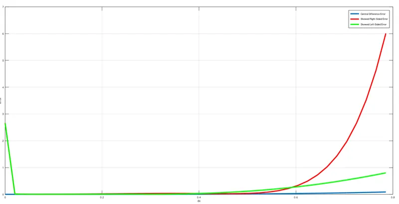
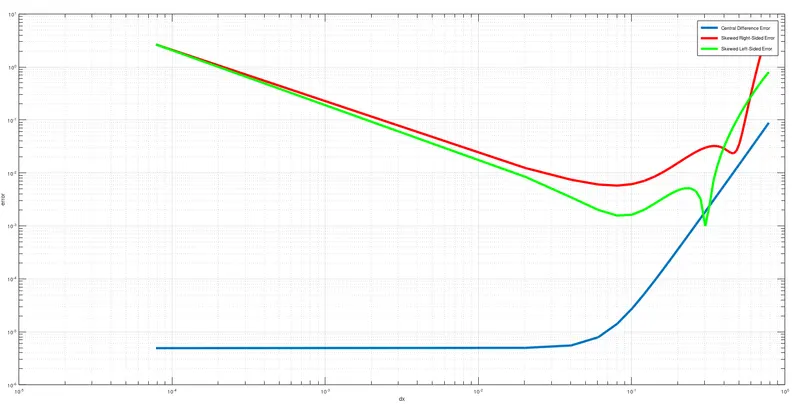
After analyzing the graph between ‘error’ vs. ‘dx’ for central, skewed right-sided, and skewed left-sided difference 4^th order error; we can easily notice that central difference approximation produces more accurate solutions; hence produces lesser errors as compared to right-skewed and left-skewed difference schemes

Since we can see that the central differencing scheme gives us more immaculate solutions or lesser errors as compared to the skewed difference scheme. But it is not always viable to use the central differencing to evaluate solutions. Suppose, if we want to compute numerical approximations for a function at the boundary or corner node; we cannot use the central difference scheme at this particular situation because it requires data from both sides of the node or boundary. So, in this situation skewed difference method plays a major role; as in the skewed scheme data from one side can be used to compute numerical approximation at a point