Week 3.5 - Deriving 4th order approximation of a 2nd order derivative using Taylor Table method

Taylor series:- It is the polynomial or a function of an infinite sum of terms. Each successive term will have a larger exponent or higher degree than the preceding term

f(x) = f(a) + f'(a)(x-a) /1! + f''(a)(x-a)² /2! + f'''(a)(x-a)³ /3! + ...

Right side skew differencing:

Here we derive the right side skew differencing for the fourth order approximation of the second order derivative of a fuction sing Taylor's table method.

for Right side skew difference

Number of Nodes, N=P+Q

here,

p=order of derivative

Q =order of approximation

N=2+4 = 6

∇x²f''(x) = af(i) +bf(i+1) cf(i+2)+df(i+3)+ef(i+4)+gf(i+5)

Evalution:

af(i) =a f(i)

bf(i+1) = b (f(i) + f'(i)(∇x) /1! + f''(i)(∇x)² /2! + f'''(i)(∇x)³ /3! + ...)

cf(i+2) = c (f(i) + f'(i)(2∇x) /1! + f''(i)(2∇x)² /2! + f'''(i)(2∇x)³ /3! + ...)

df(i+3) = d (f(i) + f'(i)(3∇x) /1! + f''(i)(3∇x)² /2! + f'''(i)(3∇x)³ /3! + ...)

ef(i+4) = e (f(i) + f'(i)(∇x) /1! + f''(i)(∇x)² /2! + f'''(i)(∇x)³ /3! + ...)

gf(i+5) = g (f(i) + f'(i)(∇x) /1! + f''(i)(∇x)² /2! + f'''(i)(∇x)³ /3! + ...)

Taylor Table:

∇x²f''(x) f(i) ∇xf'(i) ∇x²f''(i) ∇x³f'''(i) ∇x⁴f''''(i) ∇x⁵f'''''(i)

af(i) a 0 0 0 0 0

bf(i+1) b b b/2 b/6 b/24 b/120

cf(i+2) c 2c 4c/2 8c/6 16c/24 32c/120

df(i+3) d 3d 9d/2 27d/6 81d/24 243d/120

ef(i+4) e 4e 16e/2 64e/6 256e/24 1024e/120

gf(i+5) g 5g 25g/2 125g/6 625g/24 3125g/120

2nd order 0 0 1 0 0 0

derivative

from above table:

1. a+b+c+d+e+g =0

2.b+2c+3d+4e+5g =0

3.(b+4c+9d+16e+25g)/2 =1

4.(b+8c+27d+64e+125g)/6 =0

5.(b+16c+81d+256e+625g)/24 =0

6.(b+32c+243d+1024e+3125g)/120 =0

by solving the above equations we get the values of the a,b ,c,d,e,g.By use this we can find the approximation of Right side skew second order derivative for the fourth order approximation.

Left side skew differencing:

Here we derive the Left side skew differencing for the fourth order approximation of the second order derivative of a fuction sing Taylor's table method.

for Left side skew difference

Number of Nodes, N=P+Q

here,

p=order of derivative

Q =order of approximation

N=2+4 = 6

∇x²f''(x) = af(i) +bf(i-1) cf(i-2)+df(i-3)+ef(i-4)+gf(i-5)

Evalution:

af(i) =a f(i)

bf(i-1) = b (f(i) - f'(i)(∇x) /1! + f''(i)(∇x)² /2! - f'''(i)(∇x)³ /3! + ...)

cf(i-2) = c (f(i) - f'(i)(2∇x) /1! + f''(i)(2∇x)² /2! - f'''(i)(2∇x)³ /3! + ...)

df(i-3) = d (f(i) - f'(i)(3∇x) /1! + f''(i)(3∇x)² /2! - f'''(i)(3∇x)³ /3! + ...)

ef(i-4) = e (f(i) - f'(i)(∇x) /1! + f''(i)(∇x)² /2! - f'''(i)(∇x)³ /3! + ...)

gf(i-5) = g (f(i) - f'(i)(∇x) /1! + f''(i)(∇x)² /2! - f'''(i)(∇x)³ /3! + ...)

Taylor Table:

∇x²f''(x) f(i) ∇xf'(i) ∇x²f''(i) ∇x³f'''(i) ∇x⁴f''''(i) ∇x⁵f'''''(i)

af(i) a - 0 0 - 0 0 - 0

bf(i-1) b -b b/2 - b/6 b/24 -b/120

cf(i-2) c -2c 4c/2 - 8c/6 16c/24 -32c/120

df(i-3) d -3d 9d/2 -27d/6 81d/24 -243d/120

ef(i-4) e -4e 16e/2 -64e/6 256e/24 -1024e/120

gf(i-5) g -5g 25g/2 - 125g/6 625g/24 -3125g/120

2nd order 0 0 1 0 0 0

derivative

from above table:

1. a+b+c+d+e+g =0

2. - (b+2c+3d+4e+5g) =0

3.(b+4c+9d+16e+25g)/2 =1

4. -(b+8c+27d+64e+125g)/6 =0

5.(b+16c+81d+256e+625g)/24 =0

6.-(b+32c+243d+1024e+3125g)/120 =0

by solving the above equations we get the values of the a,b ,c,d,e,g.By use this we can find the approximation of Left side skew second order derivative for the fourth order approximation.

Central differencing:

Here we derive the Central differencing for the fourth order approximation of the second order derivative of a fuction sing Taylor's table method.

for Central differencing

Number of Nodes, N=P+Q-1

here,

p=order of derivative

Q =order of approximation

N=2+4 = 5

∇x²f''(x) = af(i-2)+bf(i-1)+cf(i)+df(i+1)+ef(i+2)

Evalution:

af(i-2) =a (f(i) - f'(i)(2∇x) /1! + f''(i)(2∇x)² /2! - f'''(i)(2∇x)³ /3! + ...)

bf(i-1) = b (f(i) - f'(i)(∇x) /1! + f''(i)(∇x)² /2! - f'''(i)(∇x)³ /3! + ...)

cf(i) = c f(i)

df(i+1) = d (f(i) + f'(i)(∇x) /1! + f''(i)(∇x)² /2! + f'''(i)(∇x)³ /3! + ...)

ef(i+2) = e (f(i) + f'(i)(2∇x) /1! + f''(i)(2∇x)² /2! + f'''(i)(2∇x)³ /3! + ...)

Taylor Table:

∇x²f''(x) f(i) ∇xf'(i) ∇x²f''(i) ∇x³f'''(i) ∇x⁴f''''(i)

af(i-2) a -2a 4a/2 - 8a/6 16a/24

bf(i-1) b -b b/2 - b/6 b/24

cf(i) c 0 0 0 0

df(i+1) d d d/2 d/6 d/24

ef(i+2) e 2e 4e/2 8e/6 16e/24

2nd order 0 0 1 0 0

derivative

from above table:

1. a+b+c+d+e =0

2. -2a -b +d+2e =0

3. (4a+b+d+4e)/2 =1

4. (-8a-b+d+8e)/6 =0

5. (16a+b+d+16e)/24 =0

by solving the above equations we get the values of the a,b ,c,d,e,By use this we can find the approximation of central differencing second order derivative for the fourth order approximation.

Now,we have derived all equation for the second order derviative using central differencing, right-sided differenced and left side skew differencing and we plot the result by using mathlab program.

#mathcode

clear all
close all
clc

%Given function f(x) = e^x *cosx
% analytic derivate  = -2*e^x*sinx
%let us take input x= pi/3; 
x= pi/3;
dx=linspace(pi/4000,pi/40,20);

analyticderivative = -2*exp(x)*sin(x)

%Right side skewed(RSS)
R = [1 1 1 1 1 1;
    0 1 2 3 4 5;
    0 1/2 2 9/2 16/2 25/2;
    0 1/6 8/6 27/6 64/6 125/6;
    0 1/24 16/24 81/24 256/24 625/24;
    0 1/120 32/120 243/120 1024/120 3125/120];
S=[0;0;1;0;0;0];
RSS= inv(R)*S;

%right side skewed approximation
Right_side_skewed = (RSS(1).*exp(x).*cos(x)+RSS(2).*exp(x+dx).*cos(x+dx) ...
    +RSS(3).*exp(x+2*dx).*cos(x+dx*2)+RSS(4).*exp(x+3*dx).*cos(x+3*dx) ...
    +RSS(5).*exp(x+4*dx).*cos(x+4*dx)+RSS(6).*exp(x+5*dx).*cos(x+5*dx))./(dx.^2);
%left_side_skew (LSS)
L= [1 1 1 1 1 1;
    -0 -1 -2 -3 -4 -5;
    0 1/2 4/2 9/2 16/2 25/2;
    0 -1/6 -8/6 -27/6 -64/6 -125/6;
    0 1/24 16/24 81/24 256/24 625/24;
    0 -1/120 -32/120 -243/120 -1024/120 -3125/120];
s=[0;0;1;0;0;0];
LSS = inv(L)*s;

%left side skewed approximation
Left_side_skewed =(LSS(1).*exp(x).*cos(x)+LSS(2).*exp(x-dx).*cos(x-dx) ...
    +LSS(3).*exp(x-2*dx).*cos(x-2*dx)+LSS(4).*exp(x-3*dx).*cos(x-3*dx) ...
    +LSS(5).*exp(x-4*dx).*cos(x-4*dx) ...
    +LSS(6).*exp(x-5*dx).*cos(x-5*dx))./(dx.^2);

%center Derivative (CDD)
C=[1 1 1 1 1;-2 -1 0 1 2;4/2 1/2 0 1/2 4/2;-8/6 -1/6 0 1/6 8/6;
    16/24 1/24 0 1/24 16/24];
D=[0;0;1;0;0];
CDD = inv(C)*D;
%center difference approximation
 Central_derivative = (CDD(1).*exp(x-2*dx).*cos(x-2*dx)+CDD(2).*exp(x-dx).*cos(x-dx)+CDD(3).*exp(x).*cos(x)+CDD(4).*exp(x+dx).*cos(x+dx) ...
    +CDD(5).*exp(x+2*dx).*cos(x+dx*2))./(dx.^2);


%finding error 
 error_in_right_side_skew =   abs(Right_side_skewed-analyticderivative);
error_in_Left_side_skew  =    abs(Left_side_skewed-analyticderivative);
error_in_center_derivative=   abs(Central_derivative-analyticderivative);

%ploting graph
figure(1)
loglog(dx,error_in_center_derivative,dx,error_in_Left_side_skew,dx,error_in_right_side_skew)
legend('error in center derivative','error in Left side skew','error in right side skew')
xlabel('dx')
ylabel('abosulte error')
title('error computation')
grid on

figure(2)
plot(dx,error_in_center_derivative,dx,error_in_Left_side_skew,dx,error_in_right_side_skew)
legend('error in center derivative','error in Left side skew','error in right side skew')
xlabel('dx')
ylabel('abosulte error')
title('error computation')
grid on

figure(3)
semilogy(dx,error_in_center_derivative,dx,error_in_Left_side_skew,dx,error_in_right_side_skew)
legend('error in center derivative','error in Left side skew','error in right side skew')
xlabel('dx')
ylabel('abosulte error')
title('error computation')
grid on

Results:

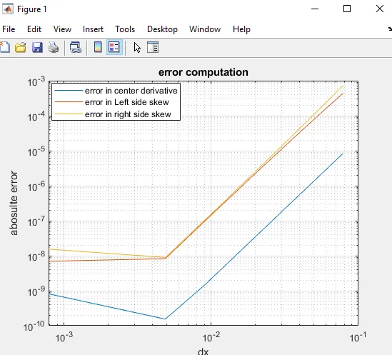
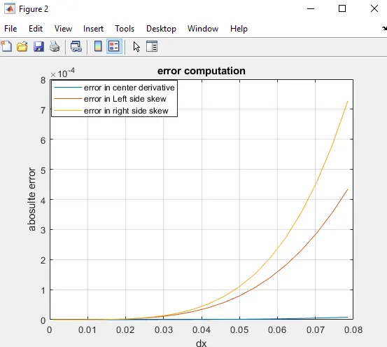
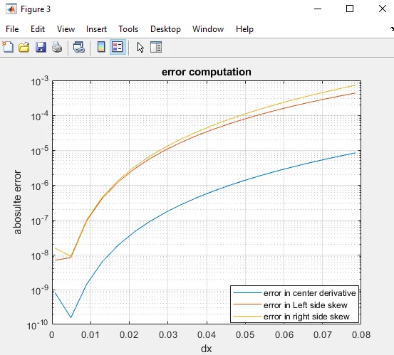
Central differencing >> Right Side Skew differencing >>Left Side Skew differencing.

skewed differencing scheme:

Skewed differecing scheme is useful beacause it is necessary to compute the grids at the corners also which central differening scheme is unable to do. symmetric nodes does not present on the corners.