Week 3.5 - Deriving 4th order approximation of a 2nd order derivative using Taylor Table method

For deriving the 4th order schemes for central difference, skewed right side difference, and left side difference we will have to write our derivative as a polynomial.

For central difference, the polynomial will look like below

`frac{del^2u}{delx^2}`= af(i-2) + bf(i-1) + cf(i) + df(i+1) + ef(i+2)

On expanding the Taylor series for each of the terms, we can form a table using the coefficients of each term up to f''''i. The table for the central difference is shown below. The order of accuracy can be checked using the following equation

The order of accuracy P = Number of nodes in the stencil N - order of derivative Q + 1 for symmetric/central schemes

For this equation, LHS is 4.

RHS = 5 - 2 +1 = 4

Hence, this is the 4th order scheme for the central difference.

Taylor Table of Central difference

	fi	`Deltax`f'i	`Deltax^2`f''i	`Deltax^3`f'''i	`Deltax^4`f''''i
af(i-2)	a	-2a	4a/2	-8a/6	16a/24
bf(i-1)	b	-b	b/2	-b/6	b/24
cf(i)	c	0	0	0	0
df(i+1)	d	d	d/2	d/6	d/24
ef(i+2)	e	2e	4e/2	8e/6	16e/24
Sum	0	0	1	0	0

For skewed right side difference, the polynomial will look like below

`frac{del^2u}{delx^2}`= af(i) + bf(i+1) + cf(i+2) + df(i+3) + ef(i+4) + g(i+5)

On expanding the Taylor series for each of the terms, we can form a table using the coefficients of each term up to f'''''i. The table for the central difference is shown below. The order of accuracy can be checked using the following equation

The order of accuracy P = Number of nodes in the stencil N - order of derivative Q for one-sided/skewed schemes

For this equation, LHS is 4.

RHS = 6 - 2 = 4

Hence, this is the 4th order scheme for the skewed right side difference

Taylor Table of Skewed right-sided difference

	fi	`Deltax`f'i	`Deltax^2`f''i	`Deltax^3`f'''i	`Deltax^4`f''''i	`Deltax^5`f'''''i
afi	a	0	0	0	0	0
bf(i+1)	b	b	b/2	b/6	b/24	b/120
cf(i+2)	c	2c	4c/2	8c/6	16c/24	32c/120
df(i+3)	d	3d	9d/2	27d/6	81d/24	243d/120
ef(i+4)	e	4e	16e/2	64e/6	256e/24	1024e/120
g(i+5)	g	5g	25g/2	125g/6	625g/24	3125g/120
Sum	0	0	1	0	0	0

For skewed left side difference, the polynomial will look like below

`frac{del^2u}{delx^2}`= af(i) + bf(i-1) + cf(i-2) + df(i-3) + ef(i-4) + g(i-5)

On expanding the Taylor series for each of the terms, we can form a table using the coefficients of each term up to f'''''i. The table for the central difference is shown below. The order of accuracy can be checked using the following equation

The order of accuracy P = Number of nodes in the stencil N - order of derivative Q for one-sided/skewed schemes

For this equation, LHS is 4.

RHS = 6 - 2 = 4

Hence, this is the 4th order scheme for the skewed left side difference

Taylor Table of Skewed left-sided difference

	fi	`Deltax`f'i	`Deltax^2`f''i	`Deltax^3`f'''i	`Deltax^4`f''''i	`Deltax^5`f'''''i
afi	a	0	0	0	0	0
bf(i+1)	b	-b	b/2	-b/6	b/24	-b/120
cf(i+2)	c	-2c	4c/2	-8c/6	16c/24	-32c/120
df(i+3)	d	-3d	9d/2	-27d/6	81d/24	-243d/120
ef(i+4)	e	-4e	16e/2	-64e/6	256e/24	-1024e/120
g(i+5)	g	-5g	25g/2	-125g/6	625g/24	-3125g/120
Sum	0	0	1	0	0	0

To calculate these schemes, different functions were written as defined below.

function for 4th order approximation of Central difference

function central_difference = fourth_order_central_difference(x, dx)
 
%matrix from system of equation from taylor table
 A = [1 1 1 1 1 ;
     -2 -1 0 1 2 ; 
     4/2 1/2 0 1/2 4/2;
     -8/6 -1/6 0 1/6 8/6;
     16/24 1/24 0 1/24 16/24];
 
 B = [0; 0; 1; 0; 0];
 
 C = A\B;
 
 %using coefficient from matrix C for finding the central difference 
 
 central_difference = (C(1)*(exp(x - (2*dx))*cos(x - (2*dx))) + C(2)*(exp(x-dx)*cos(x-dx)) + C(3)*(exp(x)*cos(x)) + C(4)*(exp(x+dx)*cos(x+dx)) + C(5)*(exp(x + (2*dx))*cos(x + (2*dx))))/((dx)^2);
 

end

function for 4th order approximation of Skewed right-sided difference

function right_side_difference = fourth_order_skewed_right(x, dx)
 
%matrix from system of equation from taylor table
 A = [1 1 1 1 1 1;
     0 1 2 3 4 5; 
     0 1/2 4/2 9/2 16/2 25/2; 
     0 1/6 8/6 27/6 64/6 125/6;
     0 1/24 16/24 81/24 256/24 625/24; 
     0 1/120 32/120 243/120 1024/120 3125/120];
 
 B = [0; 0; 1; 0; 0; 0];
 
 C = A\B;
 
 %using coefficient from matrix C for finding the right side skewed difference 

 right_side_difference = (C(1)*(exp(x)*cos(x)) + C(2)*(exp(x+dx)*cos(x+dx)) + C(3)*(exp(x + (2*dx))*cos(x + (2*dx))) + C(4)*(exp(x + (3*dx))*cos(x + (3*dx))) + C(5)*(exp(x + (4*dx))*cos(x + (4*dx))) + C(6)*(exp(x + (5*dx))*cos(x + (5*dx))))/((dx)^2);

end

function for 4th order approximation of Skewed left-sided difference

function left_side_difference = fourth_order_skewed_left(x, dx)
 
%matrix from system of equation from taylor table
 A = [1 1 1 1 1 1;
     0 -1 -2 -3 -4 -5; 
     0 1/2 4/2 9/2 16/2 25/2; 
     0 -1/6 -8/6 -27/6 -64/6 -125/6;
     0 1/24 16/24 81/24 256/24 625/24; 
     0 -1/120 -32/120 -243/120 -1024/120 -3125/120];
 
 B = [0; 0; 1; 0; 0; 0];
 
 C = A\B;
 
 %using coefficient from matrix C for finding the left side skewed difference 

 left_side_difference = (C(1)*(exp(x)*cos(x)) + C(2)*(exp(x-dx)*cos(x-dx)) + C(3)*(exp(x - (2*dx))*cos(x - (2*dx))) + C(4)*(exp(x - (3*dx))*cos(x - (3*dx))) + C(5)*(exp(x - (4*dx))*cos(x - (4*dx))) + C(6)*(exp(x - (5*dx))*cos(x - (5*dx))))/((dx)^2);

end

Main Code

clear all
close all
clc
 
%analytical function  = exp(x)*cos(x)
 

%analytical derivative
%f'(x) = exp(x)*(cos(x) - sin(x))

x = pi/3;
 
dx = linspace(pi/4000,pi/4,2000);
 
analytical_derivative = -2*exp(x)*sin(x);

skewed_right_scheme = zeros(1,2000);
skewed_left_scheme = zeros(1,2000);
central_difference_scheme = zeros(1,2000);

for i = 1:length(dx)
%Skewed right-sided difference
skewed_right_scheme(i) = fourth_order_skewed_right(x, dx(i));

%Skewed left-sided difference
skewed_left_scheme(i) = fourth_order_skewed_left(x, dx(i));

%Central difference 
central_difference_scheme(i) = fourth_order_central_difference(x, dx(i));
end
 
 
%calculating the error
error_skewed_right_scheme = abs(skewed_right_scheme - analytical_derivative);
 
error_skewed_left_scheme = abs(skewed_left_scheme - analytical_derivative);

error_central_difference_scheme = abs(central_difference_scheme - analytical_derivative);
 

figure(1)
loglog (dx, error_central_difference_scheme,'b','Linewidth',1.5)
hold on 
loglog (dx, error_skewed_right_scheme,'r','Linewidth',1.5)
loglog (dx, error_skewed_left_scheme,'g','Linewidth',1.5)
grid on
legend('Central Difference of 4th order','Skewed right sided difference of 4th order','Skewed left sided difference of 4th order')
legend('Location','northwest')
xlabel('Range of dx','FontSize',14)
ylabel('Error Value','FontSize',14)
saveas(gcf,'error_log_plot.png');  
 

The above code plots the following figure for comparing the error between the three 4th order schemes.

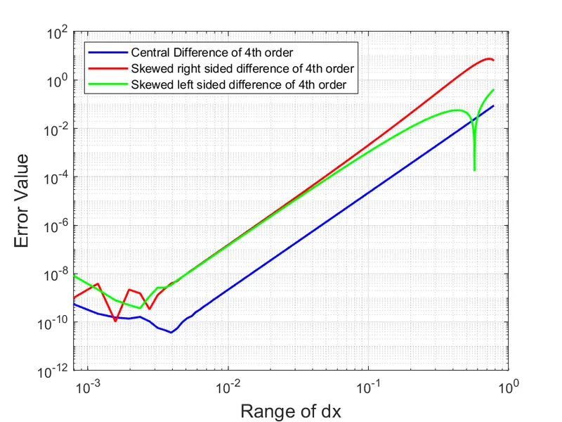
It can be seen from the plot above that the central difference scheme on average has lower error values than skewed right or skewed left schemes. We can also see that as the mesh size is reduced after a certain limit the error increases for all three schemes. This is happening due to roundoff errors as the computers have limits on their ability to store numbers.

We can also say that in most cases, the central difference scheme will be sufficient. However, central difference schemes can't be applied at boundaries. This is because the scheme requires values on both sides of the central node. This problem is alleviated by the right and left-skewed schemes and will be used on the left and right boundaries respectively.