Week 11 - Simulation of Flow through a pipe in OpenFoam
Objective of the project: 1.The main objective of this project is to simulate the laminar flow through pipe. The wedge portion is taken as the whole circular section (cylinder) may take time to simulate or it may be costly if your computer do not have much resources.
2. The other objectives is to write the Matlab code for blockMeshDict file for different wedge angle , length and radius.
3. The final objective is to post process the results of velocity at different length of the pipe and shear stress at the fully developed portion and to compare it with the analytical solution i.e by hagen poiseuille equation
Assumptions made :
- Steady flow , incompressible and laminar flow
- Flow is two dimenional ( Flow WRT theta is ignored )
- Constant fluid properties (Viscosity , Density etc)
Introduction to the laminar flow through pipe:
In this project we aim to simulate a section of pipe (Wedge shaped geometry) to understand various aspects of flow through a pipe. The fluid chosen is water and the flow is laminar and incompressible. Also we choose to neglect any changes in cross section. The specified Reynolds Number Re is specified as 2100.
Internal flow occurs when the fluid is filled entirely in a conduit and is driven primarily by a pressure difference.
Fluid velocity in a pipe changes from zero at the surface because of the no-slip boundary condition to a maximum at the pipe center. The average velocity remains constant in an incompressible flow when the cross section of the pipe is constant.
Renold's Number(Re): The transition from laminar flow to turbulent flow occurs from laminar(Re ≤">≤2100) to Transition(2100≤">≤Re≤">≤4000) to turbulent (Re≥">≥4000) for smooth pipewith no viscous dissipation. it depends on the geometry,face roughness, flow velocity,surface temperature etc.
Hydrodynamic entry length: The region from the pipe inlet to the point at which the velocity boundary layer merges at the centreline is called the hydrodynamic entrance region. The region beyond the entrance region in which the velocity profile is fully developed is called the fully developed region.
Hagen Poiseuille Flow: It states that 'for a specified flowrate, the pressure dop and thus the required pumping power is inversely proportional to the length of the pipe and the viscosity of the fluid, but it is inversely proportional to the fourth power of the radius (or diameter) of the pipe'.
- Re = 2100 (essentially laminar)
- Working fluid water : Kinematic viscosity = 8.9e-07 m^2/s
- Dynamic viscosity of the water : mu = 8.9e-04 Pa.S`
- Density of water = 1000 Kg/m^3
- Diameter of the pipe D = 0.02 m (Assuming )
MATLAB PROGRAM
In this project we have used MATLAB to write a program that will generate the mesh file (blockMeshDict file) for OpenFOAM. The geometry used is wedge made out of a single block and for different wedge angles our MATLAB program creates the required blockMeshDict file.
%simulation of flow through pipe
%creating blockmeshdict file

clear all
close all
clc

% Inputs parameters

%Reynold's number
Re = 2100;

%Density
rho = 1000;

%Diameter (in m)
D = 0.02;

%Radius
R = D/2;

%Entry Length of the pipe
L_ent = 0.06*Re*D;

%viscosity (pa.s)
mu = 0.00089;

%Kinematic Viscosity
nu = mu/rho;
%Angle of wedge
theta = 3;

%Boundary conditions
v_avg = Re*nu/D;
v_max = 2*v_avg;
L_d = 0.3;
L = L_ent + L_d;
deltap = (8*v_avg*mu*L_d)/R^2;
deltap = deltap/rho;

%vertices cordinate
v0 = [0 0 0];  %point 0
v1 = [0 R*cosd(theta/2) -R*sind(theta/2)];  %point 1
v2 = [0 R*cosd(theta/2) R*sind(theta/2)];  %point 2
v3 = [L 0 0];  %point 3
v4 = [L R*cosd(theta/2) -R*sind(theta/2)]; %point 4
v5 = [L R*cosd(theta/2) R*sind(theta/2)]; %point 5

fileid = fopen('BlockMeshDict','w')

fprintf(fileid,'FoamFile\n{\n\')
fprintf(fileid,'%12s \t 2.0;\n\','version')
fprintf(fileid,'%12s \t ascii;\n\','format')
fprintf(fileid,'%12s \t dictionary;\n\','class')
fprintf(fileid,'%12s \t blockMeshDict;\n\','object')
fprintf(fileid, '}\n\')
fprintf(fileid, 'vertices\n')
fprintf(fileid, '(\n')
fprintf(fileid, '\t(%s)\n', num2str(v0))
fprintf(fileid, '\t(%s)\n', num2str(v1))
fprintf(fileid, '\t(%s)\n', num2str(v2))
fprintf(fileid, '\t(%s)\n', num2str(v3))
fprintf(fileid, '\t(%s)\n', num2str(v4))
fprintf(fileid, '\t(%s)\n', num2str(v5))
fprintf(fileid, ');\n')

fprintf(fileid, 'blocks\n')
fprintf(fileid, '(\n')
fprintf(fileid, '\t hex (0 3 5 2 0 3 4 1) (%d %d %d)\',300,30,1)
fprintf(fileid, ' SimpleGrading (1 0.1 1)\n\n\')
fprintf(fileid, ');\n')

fprintf(fileid, 'edges\n')
fprintf(fileid, '(\n')
fprintf(fileid, '\t arc %d %d (%d %d %d)\n',1,2,0,R,0)
fprintf(fileid, '\t arc %d %d (%d %d %d)\n',4,5,L,R,0)
fprintf(fileid, ');\n')

fprintf(fileid, 'boundary\n')
fprintf(fileid, '(\n')
fprintf(fileid, '\t inlet \n')
fprintf(fileid, '\t {\n')
fprintf(fileid, '\t\t type patch;\n')
fprintf(fileid, '\t\t faces\n')
fprintf(fileid, '\t\t (\n')
fprintf(fileid, '\t\t\t (0 1 2 0)\n')
fprintf(fileid, '\t\t );\n')
fprintf(fileid, '\t }\n')

fprintf(fileid, '\t outlet\n')
fprintf(fileid, '\t {\n')
fprintf(fileid, '\t\t type patch;\n')
fprintf(fileid, '\t\t faces\n')
fprintf(fileid, '\t\t (\n')
fprintf(fileid, '\t\t\t (3 5 4 3)\n')
fprintf(fileid, '\t\t );\n')
fprintf(fileid, '\t }\n')

fprintf(fileid, '\t top\n')
fprintf(fileid, '\t {\n')
fprintf(fileid, '\t\t type wall;\n')
fprintf(fileid, '\t\t faces\n')
fprintf(fileid, '\t\t (\n')
fprintf(fileid, '\t\t\t (1 4 5 2)\n')
fprintf(fileid, '\t\t );\n')
fprintf(fileid, '\t }\n')

fprintf(fileid, '\t front\n')
fprintf(fileid, '\t {\n')
fprintf(fileid, '\t\t type wedge;\n')
fprintf(fileid, '\t\t faces\n')
fprintf(fileid, '\t\t (\n\')
fprintf(fileid, '\t\t\t (0 3 4 1)\n')
fprintf(fileid, '\t\t );\n')
fprintf(fileid, '\t }\n')

fprintf(fileid, '\t back\n')
fprintf(fileid, '\t {\n')
fprintf(fileid, '\t\t type wedge;\n')
fprintf(fileid, '\t\t faces\n')
fprintf(fileid, '\t\t (\n')
fprintf(fileid, '\t\t\t (0 2 5 3)\n')
fprintf(fileid, '\t\t );\n')
fprintf(fileid, '\t }\n')

fprintf(fileid, '\t axis\n')
fprintf(fileid, '\t {\n')
fprintf(fileid, '\t\t type empty;\n')
fprintf(fileid, '\t\t faces\n')
fprintf(fileid, '\t\t (\n')
fprintf(fileid, '\t\t\t (0 3 3 0)\n')
fprintf(fileid, '\t\t );\n')
fprintf(fileid, '\t }\n')
fprintf(fileid, '); \n\n')

fprintf(fileid, 'mergePatchPairs\n')
fprintf(fileid, '(\n')
fprintf(fileid, ');\n')

fclose(fileid)
BlockMeshDict
FoamFile
{
     version 	 2.0;
      format 	 ascii;
       class 	 dictionary;
      object 	 blockMeshDict;
}
vertices
(
	(0  0  0)
	(0   0.0099966 -0.00026177)
	(0   0.0099966  0.00026177)
	(2.82           0           0)
	(2.82   0.0099966 -0.00026177)
	(2.82   0.0099966  0.00026177)
);
blocks
(
	 hex (0 3 4 1 0 3 5 2) (300 30 1) SimpleGrading (1 0.1 1)

);
edges
(
	 arc 1 2 (0 1.000000e-02 0)
	 arc 4 5 (2.820000e+00 1.000000e-02 0)
);
boundary
(
	 inlet
	 {
		 type patch;
		 faces
		 (
			 (0 2 1 0)
		 );
	 }
	 outlet
	 {
		 type patch;
		 faces
		 (
			 (3 4 5 3)
		 );
	 }
	 top
	 {
		 type wall;
		 faces
		 (
			 (1 2 5 4)
		 );
	 }
	 front
	 {
		 type wedge;
		 faces
		 (
			 (0 3 5 2)
		 );
	 }
	 back
	 {
		 type wedge;
		 faces
		 (
			 (0 1 4 3)
		 );
	 }
	 axis
	 {
		 type empty;
		 faces
		 (
			 (0 3 3 0)
		 );
	 }
);

mergePatchPairs
(
);
ControlDict
/*--------------------------------*- C++ -*----------------------------------*\
  =========                 |
  \\      /  F ield         | OpenFOAM: The Open Source CFD Toolbox
   \\    /   O peration     | Website:  https://openfoam.org
    \\  /    A nd           | Version:  8
     \\/     M anipulation  |
\*---------------------------------------------------------------------------*/
FoamFile
{
    version     2.0;
    format      ascii;
    class       dictionary;
    location    "system";
    object      controlDict;
}
// * * * * * * * * * * * * * * * * * * * * * * * * * * * * * * * * * * * * * //

application     icoFoam;

startFrom       latestTime; // startTime

startTime       0;

stopAt          endTime;

endTime         25;

deltaT          0.02;

writeControl    runTime; //timeStep - it will print an output file every writeInterval*deltaT
			 //runTime - writes an output file every specified writeInterval sec
writeInterval   0.5;

purgeWrite      10; // 0 - it retain all the output folders

writeFormat     ascii;

writePrecision  6;

writeCompression off;

timeFormat      general;

timePrecision   6;

runTimeModifiable true;


// ************************************************************************* //
Velocity File inside zero folder
/*--------------------------------*- C++ -*----------------------------------*\
  =========                 |
  \\      /  F ield         | OpenFOAM: The Open Source CFD Toolbox
   \\    /   O peration     | Website:  https://openfoam.org
    \\  /    A nd           | Version:  8
     \\/     M anipulation  |
\*---------------------------------------------------------------------------*/
FoamFile
{
    version     2.0;
    format      ascii;
    class       volVectorField;
    object      U;
}
// * * * * * * * * * * * * * * * * * * * * * * * * * * * * * * * * * * * * * //

dimensions      [0 1 -1 0 0 0 0];

internalField   uniform (0.0934 0 0);

boundaryField
{
    inlet
    {
        type            fixedValue;
        value           uniform (0.0934 0 0);
    }

    outlet
    {
        type            zeroGradient;
    }
    top
    {
        type            noSlip;
    }
    front
    {
        type            wedge;
    }
    back
    {
        type            wedge;
    }
    axis
    {
        type            empty;
    }
}

// ************************************************************************* //
Pressure file
*--------------------------------*- C++ -*----------------------------------*\
  =========                 |
  \\      /  F ield         | OpenFOAM: The Open Source CFD Toolbox
   \\    /   O peration     | Website:  https://openfoam.org
    \\  /    A nd           | Version:  8
     \\/     M anipulation  |
\*---------------------------------------------------------------------------*/
FoamFile
{
    version     2.0;
    format      ascii;
    class       volScalarField;
    object      p;
}
// * * * * * * * * * * * * * * * * * * * * * * * * * * * * * * * * * * * * * //

dimensions      [0 2 -2 0 0 0 0];

internalField   uniform 0;

boundaryField
{
   outlet
    {
        type            fixedValue;
        value           uniform 0;
    }

    inlet
    {
        type            zeroGradient;
    }
    top
    {
        type            zeroGradient;
    }
    front
    {
        type            wedge;
    }
    back
    {
        type            wedge;
    }
    axis
    {
        type            empty;
    }
}

// ************************************************************************* //
Transport Properties
/*--------------------------------*- C++ -*----------------------------------*\
  =========                 |
  \\      /  F ield         | OpenFOAM: The Open Source CFD Toolbox
   \\    /   O peration     | Website:  https://openfoam.org
    \\  /    A nd           | Version:  8
     \\/     M anipulation  |
\*---------------------------------------------------------------------------*/
FoamFile
{
    version     2.0;
    format      ascii;
    class       dictionary;
    location    "constant";
    object      transportProperties;
}
// * * * * * * * * * * * * * * * * * * * * * * * * * * * * * * * * * * * * * //

nu              [0 2 -1 0 0 0 0] 8.9e-7;


// ************************************************************************* //
RESULTS
For wedge angle 3 degrees
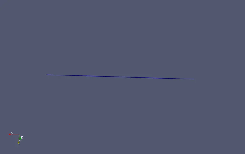
Paraview with mesh:
Post Processing
- After opening paraview click on generate to see the geometry. View the geometry from different sides across X,Y and Z axes.
- Press on the play button to post process to end time.
- Click on filters and select plot over line and plot velocity magnitude and pressure with respect to radial distance.
- Export the velocity data in .csv format.
- For calculating the shear stress import the .csv file into MATLAB
- Select the suitable column to plot shear stress.
- Write a MATLAB code to calculate shear stress.
- The shear stress should be maximum at walls.
- Plot the result for shear stress.
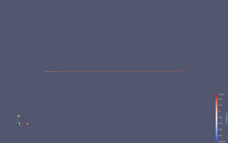
Velocity Contour
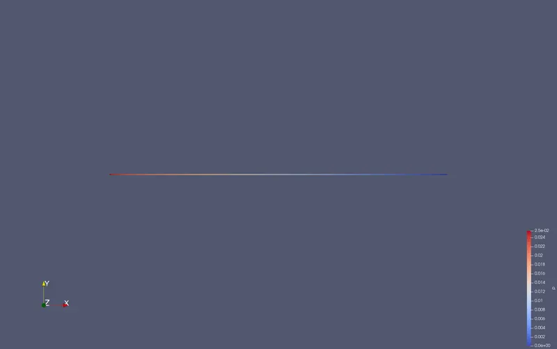
Pressure Contour
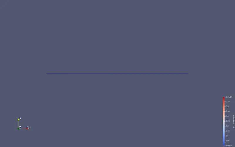
Shear stress contour
Profiles generatred
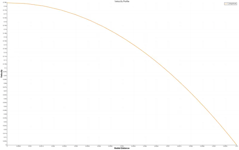
Velocity Profile
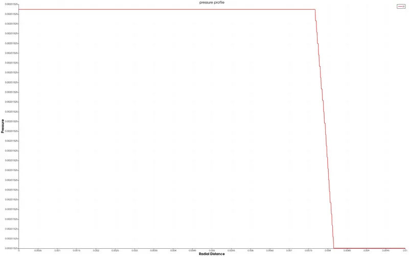
Pressure Profile
shear stress profile (tau)
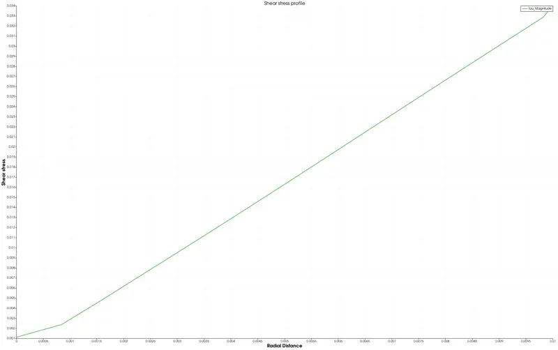
CONCLUSION
It is evident from the results that after a certain distance the parabolic velocity profile is formed and this profile remains unchanged in the axial direction which in turn tells us that the entry length we set up with respect to the conditions inside the domain is absolutely sufficient for obtaining the fully developed flow regime .Also shear stress for the fully developed flow is also plotted above.
As we can see that shear stress increases along the radius i.e shear stress is 0 at the centre of the pipe and it is maximum at the walls