Week 3.5 - Deriving 4th order approximation of a 2nd order derivative using Taylor Table method

The letter `Deltax` is used as minute amount

<No.1 Central difference(CD)>

To calculate central differene, follwoing 2 equations are used.

`f(x+Deltax)=f+f'Deltax+f^((2))frac{(Deltax)^2}{2!}+f^((3))frac{(Deltax)^3}{3!}+f^((4))frac{(Deltax)^4}{4!}+f^((5))frac{(Deltax)^5}{5!}+...`

`f(x-Deltax)=f-f'Deltax+f^((2))frac{(Deltax)^2}{2!}-f^((3))frac{(Deltax)^3}{3!}+f^((4))frac{(Deltax)^4}{4!}-f^((5))frac{(Deltax)^5}{5!}+...`

By adding those 2 equations, the result will be like this

`frac{f(x+Deltax)+f(x-Deltax)-2f}{(Deltax)^2}=f^((2))+2f^((4))frac{(2Deltax)^2}{4!}+2f^((6))frac{(2Deltax)^4}{6!}`...(1)

After repeating samethings with `f(x+2Deltax), f(x-2Deltax)`following equation is obtained

`frac{f(x+2Deltax)+f(x-2Deltax)-2f}{4(Deltax)^2}=f^((2))+2f^((4))frac{(2Deltax)^2}{4!}+2f^((6))frac{(2Deltax)^4}{6!}`...(2)

After calculating `4*(1)-(2)`, the equation for central difference is derived.

`f^((2))=frac{16f(x+Deltax)+16f(x-Deltax)-30f-f(x+2Deltax)-f(x-2Deltax)}{12(Deltax)^2}`

<No.2 Skewed right sided difference(RSD)>

To derive 4th order approximation in skewed right sided difference, terms with 5th order are needed. So Taylor series in `(x+Deltax), (x+2Deltax), (x+3Deltax), (x+4Deltax),(x+5Deltax)`are considered`

`f(x+Deltax)=f+f'Deltax+f^((2))frac{(Deltax)^2}{2!}+f^((3))frac{(Deltax)^3}{3!}+f^((4))frac{(Deltax)^4}{4!}+f^((5))frac{(Deltax)^5}{5!}+...`

`f(x+2Deltax)=f+2f'Deltax+f^((2))frac{(2Deltax)^2}{2!}+f^((3))frac{(2Deltax)^3}{3!}+f^((4))frac{(2Deltax)^4}{4!}+f^((5))frac{(2Deltax)^5}{5!}+...`

`f(x+3Deltax)=f+3f'Deltax+f^((2))frac{(3Deltax)^2}{2!}+f^((3))frac{(3Deltax)^3}{3!}+f^((4))frac{(3Deltax)^4}{4!}+f^((5))frac{(3Deltax)^5}{5!}+...`

`f(x+4Deltax)=f+4f'Deltax+f^((2))frac{(4Deltax)^2}{2!}+f^((3))frac{(4Deltax)^3}{3!}+f^((4))frac{(4Deltax)^4}{4!}+f^((5))frac{(4Deltax)^5}{5!}+...`

`f(x+5Deltax)=f+5f'Deltax+f^((2))frac{(5Deltax)^2}{2!}+f^((3))frac{(5Deltax)^3}{3!}+f^((4))frac{(5Deltax)^4}{4!}+f^((5))frac{(5Deltax)^5}{5!}+...`

Then, those equaitons are summarized in a matrix form

`((f),(f(x+Deltax)-O((Deltax)^6)),(f(x+2Deltax)-O((Deltax)^6)),(f(x+3Deltax)-O((Deltax)^6)),(f(x+4Deltax)-O((Deltax)^6)),(f(x+5Deltax)-O((Deltax)^6)))=((1,0,0,0,0,0),(1,1,frac{1}{2},frac{1}{6},frac{1}{24},frac{1}{125}),(1,2,frac{4}{2},frac{8}{6},frac{16}{24},frac{32}{125}),(1,3,frac{9}{2},frac{27}{6},frac{81}{24},frac{243}{125}),(1,4,frac{16}{2},frac{64}{6},frac{256}{24},frac{1024}{125}),(1,5,frac{25}{2},frac{125}{6},frac{625}{24},frac{3125}{125}))((f),(f'Deltax),(f''(Deltax)^2),(f^((3))(Deltax)^3),(f^((4))(Deltax)^4),(f^((5))(Deltax)^5))`...(3)

By multiplying the inverse of coefficient matrix from the left in the equation (3), the answer is obtained. The skewed right sided difference is a polynominal expression of `f, f(x+Deltax),f(x+2Deltax),f(x+3Deltax),f(x+4Deltax),f(x+5Deltax)` and the combination of coefficients is (3.75, -12.83, 17.83, -13.00, 5.08, -0.83)

<No.3 Skewed left sided difference(LSD)>

Same process as No.2 was done in skewed left sided difference. Therefore Taylor series in`(x-Deltax), (x-2Deltax), (x-3Deltax), (x-4Deltax),(x-5Deltax)` are considered and the combination of coefficients is (3.75, -12.83, 17.83, -13.00, 5.08, -0.83)

<The order of accuracy in each difference,P>

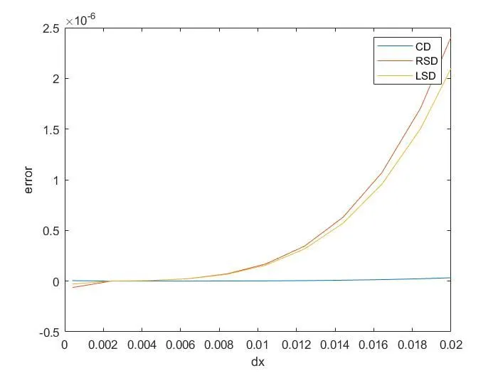
CD:P=N-Q+1=5-2+1=4

RSD:P=N-Q=6-2=4

LSD:P=N-Q=6-2=4

<Why a skewed scheme is useful? What can a skewed scheme do that a CD scheme cannot?>

One of possible usefulnesses of a skewed scheme is a situation when earlier values are not available that are necessary for CD (like x-dx or x-2dx).

<Source codes>

function[f_w35]=f_w35(x,a)
f_w35=exp(x+a)*cos(x+a);
end

clear all
close all
clc

%analytical function exp(x)*cos(x)
%numerical 2nd order derivative 2exp(x)*cosx-2exp(x)*sinx


x=1;
f=exp(x)*cos(x);
dx=linspace(pi/8000,pi/40,40);
analytical_derivative=-2*exp(x)*sin(x);


%caculate variables for skewed right sieded difference
    A_rsd=[1 0 0 0 0 0;1 1 1/2 1/6 1/24 1/120;1 2 4/2 8/6 16/24 32/120;...
        1 3 9/2 27/6 81/24 243/120;1 4 16/2 64/6 256/24 1024/120;1 5 25/2 125/6 625/24 3125/120];
    Ai_rsd=inv(A_rsd);
    rsd_mtrx1=Ai_rsd(3,:);
%caculate variables for skewed left sieded difference
    A_lsd=[1 0 0 0 0 0;1 -1 1/2 -1/6 1/24 -1/120;1 -2 4/2 -8/6 16/24 -32/120;...
        1 -3 9/2 -27/6 81/24 -243/120;1 -4 16/2 -64/6 256/24 -1024/120;1 -5 25/2 -125/6 625/24 -3125/120];
    Ai_lsd=inv(A_lsd);
    lsd_mtrx1=Ai_lsd(3,:);


%calculate 2nd order analytical derivatives
for i =1:length(dx) 
    %calculate central difference
        a_deriv_CD(i)=(16*f_w35(x,dx(i))+16*f_w35(x,-dx(i))-30*f_w35(x,0)-f_w35(x,2*dx(i))-f_w35(x,-2*dx(i)))/(12*dx(i)^2);
        error_cd(i)=analytical_derivative-a_deriv_CD(i);

    %calculate skewed right sided difference
        rsd_mtrx2=[f_w35(x,0);f_w35(x,dx(i));f_w35(x,2*dx(i));f_w35(x,3*dx(i));f_w35(x,4*dx(i));f_w35(x,5*dx(i))];
        a_deriv_rsd(i)=(rsd_mtrx1*rsd_mtrx2)/dx(i)^2;
        error_rsd(i)=analytical_derivative-a_deriv_rsd(i);
    %calculate skewed left sided difference
        lsd_mtrx2=[f_w35(x,0);f_w35(x,-dx(i));f_w35(x,-2*dx(i));f_w35(x,-3*dx(i));f_w35(x,-4*dx(i));f_w35(x,-5*dx(i))];
        a_deriv_lsd(i)=(lsd_mtrx1*lsd_mtrx2)/dx(i)^2;
        error_lsd(i)=analytical_derivative-a_deriv_lsd(i);
end

plot(dx,(error_cd));
hold on
plot(dx,(error_rsd));
hold on
plot(dx,(error_lsd));

xlim([0 0.02])
legend('CD','RSD','LSD')
xlabel('dx')
ylabel('error')

<The graph that shows errors at x=1 )