Week 3.5 - Deriving 4th order approximation of a 2nd order derivative using Taylor Table method

Problem Statement -

Derive the following 4th order approximations of the second-order derivative.

1. Central difference

2. Skewed right-sided difference

3. Skewed left-sided difference

Then write a program in Matlab to evaluate the second-order derivative of the analytical function exp(x)*cos(x) and compare it with the 3 numerical approximations that you have derived.

Provide a plot that compares the absolute error between the above-mentioned schemes

Theory -

The taylor series for the function is written as,

the above equation is valid only if:

* if the number of terms are infinite and the series converges.

* dx tends to zero

Taylor Table:

It is a method that comes up with schemes that meet the targeted accuracy.

Formulas :

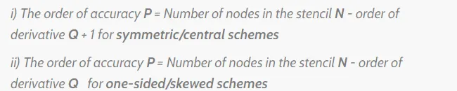
Since the order is second and the order of approximation is 4, the number of nodes in the central difference scheme is 5 and the number of nodes in skewed right sided and skewed left sided schemes are 6.

CENTRAL DIFFERENCING SCHEME:

We take up a hypothetical equation like -

Here a,b,c,d,e are coefficients. We need to find out these coefficients.

Solving Procedure-

* First we expand every term of above equation using taylor series.

* Then we put those equations in table format.The columns will represent the stencils.

* Then we use these equations to find out the unknown values.

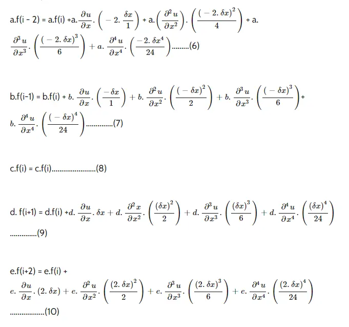
Substituting these above equations -

we get

Now writing these equations in tabular form -

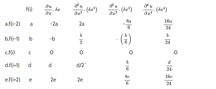
As we know the left hand of the equations only has second order derivative so all other terms can be equated to zero.

so we get-

a+b+c+d+e = 0

-2a-b+d+2e = 0

2a+b/2+d/2+2e = 1

-(8/6)*a-b/6+d/6+(8e/6)=0

(16a/24)+b/24+d/24+(16e/24)=0

Here we have 5 equations and 5 unknowns. We can solve these equations in MATLAB by putting them in a matrix form;

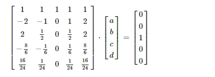
Solving for above matrix we get a = (-1/12) , b=(4/3), c=(-5/2) , d=(4/3) , e=(-1/12)

So by putting these above values in the equation we get -

SKEWED RIGHT SIDED DIFFERENCE -

The equations is:

By using taylor series expansion we get taylor table:

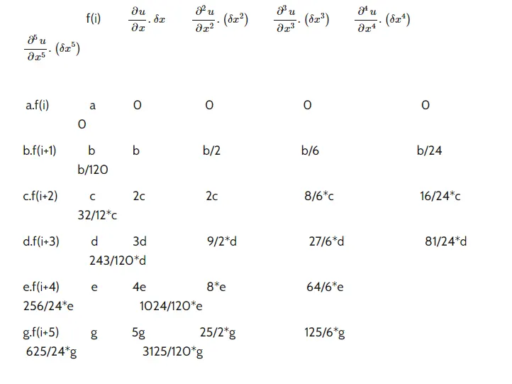
Applying same logic as we applied in central difference scheme we get the equations as -

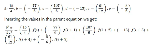
SKEWED LEFT SIDED DIFFERENCE -

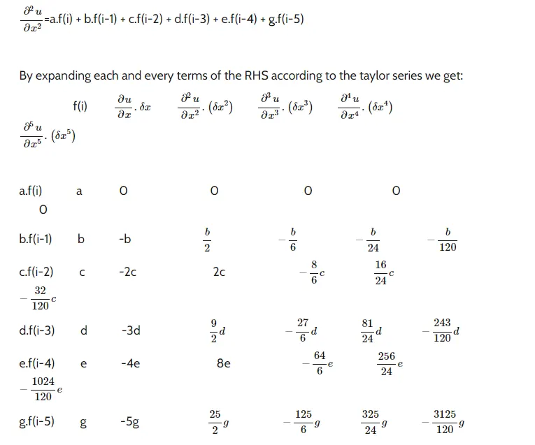
In skewed right sided differnce we condsidered descrete points at the right side but here we will consider the left side descrete points.

The equation is -

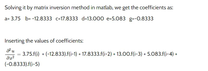
Code -

clear all
close all
clc
%analytical function = exp(x)*cos(x)
%analytical_derivative = -2*exp(x)*sin(x)
x = pi/3;
dx = linspace(pi/400,pi/4,100);
for i = 1:length(dx)
    central_difference_scheme_error(i) = central_difference(x,dx(i));
    right_skewed_scheme_error(i)=right_skewed_difference(x,dx(i));
    left_skewed_scheme_error(i)=left_skewed_difference(x,dx(i));
end
%plotting graphs
figure(1)
loglog(dx,right_skewed_scheme_error,'color','b','marker','diamond')
hold on
loglog(dx,left_skewed_scheme_error,'color','g','marker','*')
hold on 
loglog(dx,central_difference_scheme_error,'color','r','marker','.')
grid on 
xlabel('grid size')
ylabel('error')
legend('skewed right sided ' , 'skewed left sided' , 'central difference scheme')

Functions -

function central_error = central_difference(x,dx)
analytical_derivative = -2*exp(x)*sin(x);
a=(-1/12);
b=(4/3);
c=(-5/2);
d=(4/3);
e=(-1/12);
central_difference_scheme = (a*exp(x-2*dx)*cos(x-2*dx)+b*exp(x-dx)*cos(x-dx)+c*exp(x)*cos(x)+d*exp(x+dx)*cos(x+dx)+e*exp(x+2*dx)*cos(x+2*dx))/(dx^2);
central_error = abs(central_difference_scheme-analytical_derivative);
end

function right_error = right_skewed_difference(x,dx)
analytical_derivative = -2*exp(x)*sin(x);
a=(15/4);
b=(-77/6);
c=(107/6);
d=(-13);
e=(61/12);
g = (-5/6);
right_scheme = (a*exp(x)*cos(x)+b*exp(x+dx)*cos(x+dx)+c*exp(x+2*dx)*cos(x+2*dx)+d*exp(x+3*dx)*cos(x+3*dx)+e*exp(x+4*dx)*cos(x+4*dx)+g*exp(x+5*dx)*cos(x+5*dx))/(dx^2);
right_error = abs(right_scheme-analytical_derivative);
end

function left_error =left_skewed_difference(x,dx)
analytical_derivative = -2*exp(x)*sin(x);
a=(15/4);
b=(-77/6);
c=(107/6);
d=(-13);
e=(61/12);
g = (-5/6);
left_scheme = (a*exp(x)*cos(x)+b*exp(x-dx)*cos(x-dx)+c*exp(x-2*dx)*cos(x-2*dx)+d*exp(x-3*dx)*cos(x-3*dx)+e*exp(x-4*dx)*cos(x-4*dx)+g*exp(x-5*dx)*cos(x-5*dx))/(dx^2);
left_error = abs(left_scheme-analytical_derivative);
end

OUTPUT-

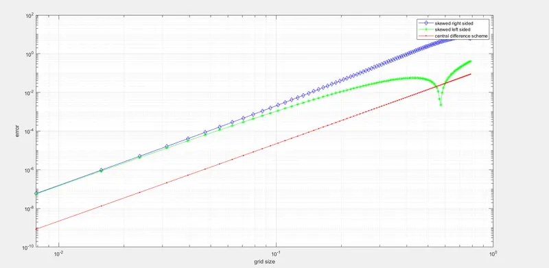
CONCLUSION -

* As we see for the same value of dx, the central scheme gives a minimum error compared to other two schemes.

* Higher order accuracy gives a more qualitative solution.