Week 3.5 - Deriving 4th order approximation of a 2nd order derivative using Taylor Table method

Deriving 4th order approximation of a 2nd order derivative using Taylor Table method

1. Central difference:

We know that, number of nodes for central scheme = order of derivative + order of approximation – 1,

No. of nodes = (2 + 4) – 1 = 5.

Therefore, the nodes required to solve a second order derivative for 4^th order central scheme approximation are (i-2), (i-1), i, (i+1), and (i+2)

∂²f/∂x² = 4^th order approximation using the nodes (i-2), (i-1), i, (i+1), and (i+2)

∆x²∂²f/∂x² = af(i-2) + bf(i-1) + cf(i) + df(i+1) + ef(i+2)

By expanding the functions at the above nodes using Taylor’s formula and arranging it in a table (Taylor’s Table), we get:

	f(i)	∆x fI(i)	∆x2 fII(i)	∆x3 fIII(i)	∆x4 fIV(i)	∆x5 fV(i)
af(i-2)	a	-2a	4a/2	-8a/6	16a/24	-32a/120
bf(i-1)	b	-b	b/2	-b/6	b/24	-b/120
cf(i)	c	0	0	0	0	0
d(i+1)	d	d	d/2	d/6	d/24	d/120
ef(i+2)	e	2e	4e/2	8e/6	16e/24	32e/120
∆x2 ∂2f/∂x2 ≈	0	0	1	0	0	?

Rewriting the sum of each row in the form of equations, we get:

a + b + c + d + e = 0;

-2a - b + 0 + d + 2e = 0;

4a/2 + b/2 + 0 + d/2 + 4e/2 = 1;

-8a/6 - b/6 + 0 + d/6 + 8e/6 = 0;

16a/24 + b/24 + 0 + d/24 + 16e/24 = 0;

(Since there are only 5 unknowns in our assumption of approximation, only the first five equations are considered to be solved so as to avoid the system from getting over-specified)

Rewriting the above equations in the form of a matrix, we get:

`[[1,1,1,1,1],[-2,-1,0,1,2],[4/(2),1/(2),0,1/(2),4/(2)],[-8/(6),-1/(6),0,1/(6),8/(6)],[16/(24),1/(24),0,1/(24),16/(24)]] [(a),(b),(c),(d),(e)] = [(0),(0),(1),(0),(0)]`

We solve the above matrix using MATLAB as:

A_central = [1 1 1 1 1;-2 -1 0 1 2;4/2 1/2 0 1/2 4/2;-8/6 -1/6 0 1/6 8/6;16/24 1/24 0 1/24 16/24];

B_central = [0;0;1;0;0];

x_central = linsolve(A_central,B_central)

x_central =

   -0.0833

    1.3333

   -2.5000

    1.3333

   -0.0833

So, the values of a, b, c, d, and e are as follows:

`[(a),(b),(c),(d),(e)] = [(-0.0833),(1.3333),(-2.5000),(1.3333),(-0.0833)]`

Substituting these values in our approximation, we get the required numerical approximation as:

∂²f/∂x² ≈ (-0.0833f(i-2) + 1.3333f(i-1) – 2.5000f(i) + 1.3333f(i+1) – 0.0833f(i+2))/ ∆x²

2. Skewed right-sided difference:

We know that, number of nodes for a Skewed scheme = order of derivative + order of approximation,

No. of nodes = 2 + 4 = 6.

Therefore, the nodes required to solve a second order derivative for a 4^th order Skewed right-sided difference scheme approximation are i, (i+1), (i+2), (i+3), (i+4) and (i+5)

∂²f/∂x² = 4^th order approximation using the nodes i, (i+1), (i+2), (i+3), (i+4) and (i+5)

∆x²∂²f/∂x² ≈ af(i) + bf(i+1) + cf(i+2) + df(i+3) + ef(i+4) + gf(i+5)

By expanding the functions at the above nodes using Taylor’s formula and arranging it in a table (Taylor’s Table), we get:

	f(i)	∆x fI(i)	∆x2 fII(i)	∆x3 fIII(i)	∆x4 fIV(i)	∆x5 fV(i)	∆x6 fVI(i)
af(i)	a	0	0	0	0	0	0
b(i+1)	b	b	b/2	b/6	b/24	b/120	b/720
cf(i+2)	c	2c	4c/2	8c/6	16c/24	32c/120	64c/720
df(i+3)	d	3d	9d/2	27d/6	81d/24	243d/120	729d/720
ef(i+4)	e	4e	16e/2	64e/6	256e/24	1024e/120	4096e/720
gf(i+5)	g	5g	25g/2	125g/6	625g/24	3125g/120	15625g/720
∆x2 ∂2f/∂x2 ≈	0	0	1	0	0	0	?

(Since there are only 6 unknowns in our assumption of approximation, only the first six equations are considered to be solved so as to avoid the system from getting over-specified)

Rewriting the above summation in the form of equations, we get:

a + b + c + d + e + g = 0

0 + b + 2c + 3d + 4e + 5g = 0

0 + b/2 + 4c/2 + 9d/2 + 16e/2 + 25g/2 = 1

0 + b/6 + 8c/6 + 27d/6 + 64e/6 + 125g/6 = 0

0 + b/24 + 16c/24 + 81d/24 + 256e/24 + 625g/24 = 0

0 + b/120 + 32c/120 + 243d/120 + 1024e/120 + 3125g/120 = 0

We solve the above equations using MATLAB as:

A_right =[1 1 1 1 1 1;0 1 2 3 4 5;0 1/2 4/2 9/2 16/2 25/2;0 1/6 8/6 27/6 64/6 125/6;0 1/24 16/24 81/24 256/24 625/24;0 1/120 32/120 243/120 1024/120 3125/120];

B_right= [0;0;1;0;0;0];

x_right = linsolve(A_right,B_right)

x_right =

    3.7500

  -12.8333

   17.8333

  -13.0000

    5.0833

   -0.8333

So, we get the values of a, b, c, d, e and g as follows:

`[(a),(b),(c),(d),(e)] = [(3.7500),( -12.8333),(17.8333),(-13.0000),(5.0833),(-0.8333)]`

Substituting these values in our approximation and dividing both sides by ∆x², we get the required approximation as:

∂²f/∂x² ≈ (3.7500f(i) – 12.8333f(i+1) + 17.8333f(i+2) – 13.0000f(i+3) + 5.0833f(i+4) – 0.8333f(i+5))/ ∆x²

3. Skewed left-sided difference:

We know that, number of nodes for a Skewed scheme = order of derivative + order of approximation,

No. of nodes = 2 + 4 = 6.

Therefore, the nodes required to solve a second order derivative for a 4^th order Skewed left-sided difference scheme approximation are (i-5), (i-4), (i-3), (i-2), (i-1), and i

∂²f/∂x² = 4^th order approximation using the nodes (i-5), (i-4), (i-3), (i-2), (i-1), and i

∆x²∂²f/∂x² ≈ af(i) + bf(i-1) + cf(i-2) + df(i-3) +ef(i-4) + gf(i-5)

By expanding the functions at the above nodes using Taylor’s formula and arranging it in a table (Taylor’s Table), we get:

	f(i)	∆x fI(i)	∆x2 fII(i)	∆x3 fIII(i)	∆x4 fIV(i)	∆x5 fV(i)	∆x6 fVI(i)
af(i)	a	0	0	0	0	0	0
bf(i-1)	b	-b	b/2	-b/6	b/24	-b/120	b/720
cf(i-2)	c	-2c	4c/2	-8c/6	16c/24	-32c/120	64c/720
df(i-3)	d	-3d	9d/2	-27d/6	81d/24	-243d/120	729d/720
ef(i-4)	e	-4e	16e/2	-64e/6	256e/24	-1024e/120	4096e/720
gf(i-5)	g	-5g	25g/2	-125g/6	625g/24	-3125g/120	15625g/720
∆x2 ∂2f/∂x2 ≈	0	0	1	0	0	0	?

(Since there are only 6 unknowns in our assumption of approximation, only the first six equations are considered to be solved so as to avoid the system from getting over-specified)

Rewriting the above summation in the form of equations, we get:

a + b + c + d + e + g = 0

0 – b – 2c – 3d – 4e – 5g = 0

0 + b/2 + 4c/2 + 9d/2 + 16e/2 + 25g/2 = 1

0 – b/6 – 8c/6 – 27d/6 – 64e/6 – 125g/6 = 0

0 + b/24 + 16c/24 + 81d/24 + 256e/24 + 625g/24 = 0

0 – b/120 – 32c/120 – 243d/120 – 1024e/120 – 3125g/120 = 0

We solve the above equations using MATLAB as:

A_left = [1 1 1 1 1 1;0 -1 -2 -3 -4 -5;0 1/2 4/2 9/2 16/2 25/2; 0 -1/6 -8/6 -27/6 -64/6 -125/6;0 1/24 16/24 81/24 256/24 625/24;0 -1/120 -32/120 -243/120 -1024/120 -3125/120];

B_left = [0;0;1;0;0;0];

x_left = linsolve(A_left,B_left)

x_left =

    3.7500

  -12.8333

   17.8333

  -13.0000

    5.0833

   -0.8333

So, the values of a, b, c, d, and e are as follows:

`[(a),(b),(c),(d),(e),(g)] = [(3.7500),(-12.8333),(17.8333),(-13.0000),(5.0833),(-0.8333)]`

Substituting these values in our approximation, we get the required approximation as:

∂²f/∂x² ≈ (3.7500f(i) – 12.8333f(i-1) + 17.8333f(i-2) – 13.0000f(i-3) + 5.0833f(i-4) – 0.8333f(i-5))/ ∆x²

4. To Prove: Skewed schemes are fourth-order accurate

Proof: In right-sided skewed scheme,

∆x² ∂²f/∂x² = af(i) + bf(i+1) + cf(i+2) + df(i+3) + ef(i+4) + gf(i+5)

all the coefficients up to f^VI(i) term vanishes except f^II(i) whose coefficient is 1 and all other higher order derivatives are neglected. Since the only terms we are left with are f^II(i) and f^VI(i) with one and unknown coefficients respectively. So, we get the approximation as:

∆x² ∂²f/∂x² = (1) ∆x² f^II(i) + (0 + b/120 + 32c/120 + 243d/120 + 1024e/120 + 3125g/120) ∆x⁶ f^VI(i)

Substituting the values of a,b,c,d,e and g in the coefficient, we get

∆x² f^II(i) + (-0.7611) ∆x⁶ f^VI(i)

Dividing both LHS and RHS by ∆x² simplifies the equation even further as below

∂²f/∂x² = f^II(i) + (-0.7611) ∆x⁴ f^VI(i) = f^II(i) + O(∆x⁴)

It implies that the skewed right sided difference scheme of a second order derivative is fourth order accurate as the truncation error O(∆x⁴) in it is of order 4. Similarly, we can show that the skewed left sided difference is also of order 4. Thus, skewed schemes are fourth order accurate. Q.E.D.

5. A MATLAB program to evaluate the second-order derivative of the analytical function exp(x)*cos(x) & its comparision with the 3 numerical approximations derived above and a plot that compares the absolute error between the above-mentioned schemes (central, right-sided skewed and left-sided skewed).

% A program that compares the absolute error between central, right-sided skewed and left-sided skewed schemes
% Approximations should be 4th order acurate and of the second-order derivative

clear all
close all
clc

% Analytical function = exp(x)*cos(x);
f = @(x) exp(x)*cos(x);
x = pi/3;
dx = linspace(pi/400,pi/4,40);

% analytical second order derivative of f
d2fdx2 = -2*exp(x)*sin(x);

% Numerical derivative
% fourth order:	Central differencing function
% ∂2f/∂x2 ≈ (af(i-2) + bf(i-1)+ cf(i) + df(i+1) + ef(i+2))/(dx^2)
A_central = [1 1 1 1 1;-2 -1 0 1 2;4/2 1/2 0 1/2 4/2;-8/6 -1/6 0 1/6 8/6;16/24 1/24 0 1/24 16/24];
B_central = [0;0;1;0;0];
R = inv(A_central)*B_central; % values of a,b,c,d and e are stored in R vector
central_diff = @(x,dx) (R(1)*f(x-2*dx) + R(2)*f(x-dx) + R(3)*f(x) + R(4)*f(x+dx) + R(5)*f(x+2*dx))/(dx^2);


% fourth order:	Skewed right-sided differencing function
% ∂2f/∂x2 ≈ (af(i) + bf(i+1) + cf(i+2) + df(i+3) + ef(i+4) + gf(i+5))/(dx^2)
A_right =[1 1 1 1 1 1;0 1 2 3 4 5;0 1/2 4/2 9/2 16/2 25/2;0 1/6 8/6 27/6 64/6 125/6;0 1/24 16/24 81/24 256/24 625/24;0 1/120 32/120 243/120 1024/120 3125/120];
B_right= [0;0;1;0;0;0];
S = inv(A_right)*B_right; % values of a,b,c,d,e and g are stored in S vector
skewed_right_diff = @(x,dx) (S(1)*f(x) + S(2)*f(x+dx) + S(3)*f(x+2*dx) + S(4)*f(x+3*dx) + S(5)*f(x+4*dx) + S(6)*f(x+5*dx))/(dx^2);

% fourth order:	Skewed left-sided differencing function
% ∂2f/∂x2 ≈ (af(i) + bf(i-1) + cf(i-2) + df(i-3) +ef(i-4) + gf(i-5))/(dx^2)
A_left = [1 1 1 1 1 1;0 -1 -2 -3 -4 -5;0 1/2 4/2 9/2 16/2 25/2; 0 -1/6 -8/6 -27/6 -64/6 -125/6;0 1/24 16/24 81/24 256/24 625/24;0 -1/120 -32/120 -243/120 -1024/120 -3125/120];
B_left = [0;0;1;0;0;0];
T = inv(A_left)*B_left; % values of a,b,c,d,e and g are stored in T vector
skewed_left_diff = @(x,dx) (T(1)*f(x) + T(2)*f(x-dx) + T(3)*f(x-2*dx) + T(4)*f(x-3*dx) + T(5)*f(x-4*dx) + T(6)*f(x-5*dx))/(dx^2); 

% Error calculation
for i = 1:length(dx)
    central_diff_error(i) = abs(d2fdx2-central_diff(x,dx(i)));
    skewed_right_error(i) = abs(d2fdx2-skewed_right_diff(x,dx(i)));
    skewed_left_error(i) = abs(d2fdx2-skewed_left_diff(x,dx(i)));
end

% plotting
loglog(dx,central_diff_error,"b-d")
hold on
loglog(dx,skewed_right_error,"k-s","LineWidth",1)
loglog(dx,skewed_left_error,"r-o","LineWidth",1.2)
hold off
xlabel("Values of dx")
ylabel("Absolute Error")
legend("central diff error","skewed right sided error","skewed left sided error","Location","northwest")
title("Range of dx vs Absolute Error plot");

The output is as follows:

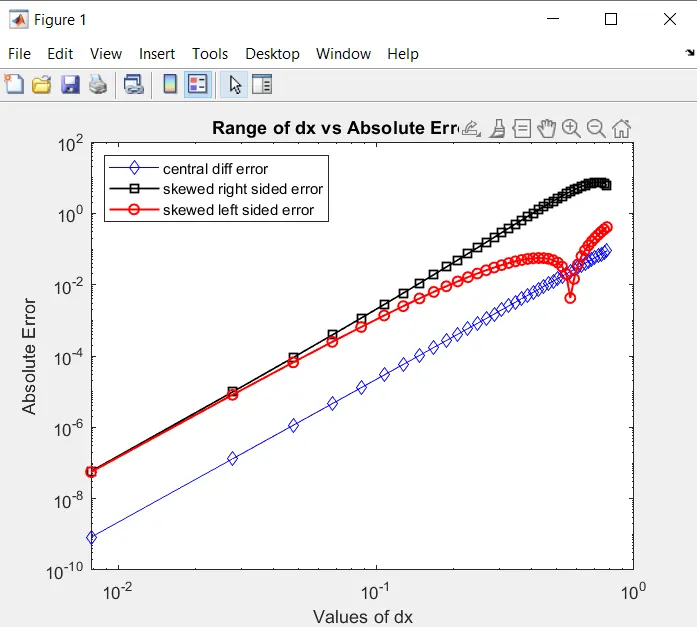
Conclusion: It is clear from the output plot that central differencing has the least absolute error hence it is the most accurate among all the schemes because it has a truncation error of second order O(∆x²) which provides more accuracy in approximation of the first derivative but it also requires the information from both sides (front and back) of the node. In most of the situation we only know the values of a function in one particular direction. So, it is not practical to use central differecning in all the scenarios. That is why we often use skewed schemes.