Week 3.5 - Deriving 4th order approximation of a 2nd order derivative using Taylor Table method

Aim:

To derive the following 4th order approximations of the second-order derivative (exp(x)*cos(x))

1. Central difference

2. Skewed right-sided difference

3. Skewed left-sided difference

Hint:

symmetric/central scheme

P =N-Q+1 so N = P+Q-1

one-sided/skewed scheme

P = N-Q so N = P+Q

where N = Number of nodes in the stencil;

P = Order of approximation

Q = Order of derivative

Solution:

Function= exp(x)*cos(x)

Analytical second order derivative = -2*exp(x)*sin(x)

Centeral Differencing:

No. of nodes = P+Q-1 =4+2-1 = 5

`(d²y)/(dx²) = (a*f(i-2)+b*f(i-1)+c*f(i)+d*f(i+1)+e*f(i+2))/(dx²)` ---> equation1

`a*f(i-2)= a[f(i)-(2deltax)/(1!)*f'(i)+(2deltax²)/(2!)*f''(i)-(2deltax³)/(3!)*f'''(i)+(2deltax^4)/(4!)*f''''(i)]`

`b*f(i-1)= b[f(i)-(deltax)/(1!)*f'(i)+(deltax²)/(2!)*f''(i)-(deltax³)/(3!)*f'''(i)+(deltax^4)/(4!)*f''''(i)]`

`c*f(i)= c[f(i)]`

`d*f(i+1)= d[f(i)+(deltax)/(1!)*f'(i)+(deltax²)/(2!)*f''(i)+(deltax³)/(3!)*f'''(i)+(deltax^4)/(4!)*f''''(i)]`

`e*f(i-2)= e[f(i)+(2deltax)/(1!)*f'(i)+(2deltax²)/(2!)*f''(i)+(2deltax³)/(3!)*f'''(i)+(2deltax^4)/(4!)*f''''(i)]`

Co-efficient Matrix

[1 1 1 1 1; -2 -1 0 1 2; 4/2 1/2 0 1/2 4/2; -8/6 -1/6 0 1/6 8/6; 16/24 1/24 0 1/24 16/24]

Constants =[a_cd;b_cd;c_cd;e_cd; f_cd]

Sum of co-efficents =[0;0;1;0;0] --> due to second order derrivative

`[Co-efficient Matrix]*[Constants] = [Sum of co-efficients]`

`Constants = Inv (Co-efficient Matrix)* Sum of co-efficients`

So

a_cd = -0.083333333333333

b_cd = 1.333333333333334

c_cd = -2.500000000000001

d_cd = 1.333333333333334

e_cd = -0.083333333333333

With the above constants and using equation 1 calculate the Central differencing approximation and subtract from Analytical derrivative to calculate the 4th order central differencing error.

Skewed right side difference:

No. of nodes = P+Q =4+2 = 6

`(d²y)/(dx²) = (a*f(i)+b*f(i+1)+c*f(i+2)+d*f(i+3)+e*f(i+4)+g*f(i+5))/(dx²)`--->equation2

`a*f(i)= a[f(i)]`

`b*f(i+1)= b[f(i)+(deltax)/(1!)*f'(i)+(deltax²)/(2!)*f''(i)+(deltax³)/(3!)*f'''(i)+(deltax^4)/(4!)*f''''(i)+(deltax^5)/(5!)*f'''''(i)]`

`c*f(i+2)= c[f(i)+(2*deltax)/(1!)*f'(i)+(2*deltax²)/(2!)*f''(i)+(2*deltax³)/(3!)*f'''(i)+(2*deltax^4)/(4!)*f''''(i)+(2*deltax^5)/(5!)*f'''''(i)]`

`d*f(i+3)= d[f(i)+(3*deltax)/(1!)*f'(i)+(3*deltax²)/(2!)*f''(i)+(3*deltax³)/(3!)*f'''(i)+(3*deltax^4)/(4!)*f''''(i)+(3*deltax^5)/(5!)*f'''''(i)]`

`e*f(i+4)= e[f(i)+(4*deltax)/(1!)*f'(i)+(4*deltax²)/(2!)*f''(i)+(4*deltax³)/(3!)*f'''(i)+(4*deltax^4)/(4!)*f''''(i)+(4*deltax^5)/(5!)*f'''''(i)]`

`g*f(i+5)= g[f(i)+(5*deltax)/(1!)*f'(i)+(5*deltax²)/(2!)*f''(i)+(5*deltax³)/(3!)*f'''(i)+(5*deltax^4)/(4!)*f''''(i)+(5*deltax^5)/(5!)*f'''''(i)]`

Co-efficient Matrix =

[1 1 1 1 1 1; 0 1 2 3 4 5; 0 1/2 4/2 9/2 16/2 25/2; 0 1/6 8/6 27/6 64/6 125/6; 0 1/24 16/24 81/24 256/24 652/24; 0 1/120 32/120 243/120 1024/120 3125/120];

Constants= [a_sr;b_sr;c_sr;e_sr; f_sr]

Sum of co-efficents =[0;0;1;0;0;0] --> due to second order derrivative

`[Co-efficient Matrix]*[Constants] = [Sum of co-efficients]`

`Constants = Inv (Co-efficient Matrix)* Sum of co-efficients`

So

a_sr = 3.750000000000011

b_sr = -12.833333333333377

c_sr = 17.833333333333420

d_sr = -13.000000000000087

e_sr = 5.083333333333376

g_sr = -0.833333333333341

With the above constants and using equation 2 calculate the skewed right approximation and subtract from Analytical derrivative to calculate the 4th order skewed right error.

Skewed left side difference:

No. of nodes = P+Q =4+2 = 6

`(d²y)/(dx²) = (a*f(i-5)+b*f(i-4)+c*f(i-3)+d*f(i-2)+e*f(i-1)+g*f(i))/(dx²)`--->equation3

`a*f(i-5)= a[f(i)-(5*deltax)/(1!)*f'(i)+(5*deltax²)/(2!)*f''(i)-(5*deltax³)/(3!)*f'''(i)+(5*deltax^4)/(4!)*f''''(i)-(5*deltax^5)/(5!)*f'''''(i)]`

`b*f(i-4)= b[f(i)-(4*deltax)/(1!)*f'(i)+(4*deltax²)/(2!)*f''(i)-(4*deltax³)/(3!)*f'''(i)+(4*deltax^4)/(4!)*f''''(i)-(4*deltax^5)/(5!)*f'''''(i)]`

`c*f(i-3)= c[f(i)-(3*deltax)/(1!)*f'(i)+(3*deltax²)/(2!)*f''(i)-(3*deltax³)/(3!)*f'''(i)+(3*deltax^4)/(4!)*f''''(i)-(3*deltax^5)/(5!)*f'''''(i)]`

`d*f(i-2)= d[f(i)-(2*deltax)/(1!)*f'(i)+(2*deltax²)/(2!)*f''(i)-(2*deltax³)/(3!)*f'''(i)+(2*deltax^4)/(4!)*f''''(i)-(2*deltax^5)/(5!)*f'''''(i)]`

`e*f(i-1)= e[f(i)-(deltax)/(1!)*f'(i)+(deltax²)/(2!)*f''(i)-(deltax³)/(3!)*f'''(i)+(deltax^4)/(4!)*f''''(i)-(deltax^5)/(5!)*f'''''(i)]`

`g*f(i)= g[f(i)]`

Co-efficient Matrix =

[1 1 1 1 1 1; -5 -4 -3 -2 -1 0; 25/2 16/2 9/2 4/2 1/2 0; -125/6 -64/6 -27/6 -8/6 -1/6 0; 625/24 256/24 81/24 16/24 1/24 0; -3125/120 -1021/120 -243/120 -32/120 -1/120 0]

Constants =[a_sl;b_sl;c_sl;e_sl; f_sl]

Sum of co-efficents =[0;0;1;0;0;0] --> due to second order derrivative

`[Co-efficient Matrix]*[Constants] = [Sum of co-efficients]`

`Constants = Inv (Co-efficient Matrix)* Sum of co-efficients`

So

a_sl = -0.833333333333337

b_sl = 5.083333333333354

c_sl = -13.000000000000032

d_sl = 17.833333333333343

e_sl = -12.833333333333314

g_sl = 3.749999999999989

With the above constants and using equation 3 calculate the skewed left approximation and subtract from Analytical derrivative to calculate the 4th order skewed left error.

Matlab Code:

close all
clear all
clc

x=pi/3;
dx=linspace(pi/500,pi/5,60);

% Central Differencing Method:
CD_Coefficients=[1 1 1 1 1; -2 -1 0 1 2; 4/2 1/2 0 1/2 4/2;...
                 -8/6 -1/6 0 1/6 8/6; 16/24 1/24 0 1/24 16/24];

CD_sum_Coefficents =[0;0;1;0;0];

CD_Constants= inv(CD_Coefficients)*CD_sum_Coefficents;


a_cd=CD_Constants(1);
b_cd=CD_Constants(2);
c_cd=CD_Constants(3);
d_cd=CD_Constants(4);
e_cd=CD_Constants(5);

% Skewed Right Sceme:
Skewed_Right_Coefficients=[1 1 1 1 1 1;...
                           0 1 2 3 4 5;...
                           0 1/2 4/2 9/2 16/2 25/2;...
                           0 1/6 8/6 27/6 64/6 125/6;...
                           0 1/24 16/24 81/24 256/24 625/24;...
                           0 1/120 32/120 243/120 1024/120 3125/120];


Skewed_Right_Sum_Coefficents =[0;0;1;0;0;0];

Skewed_Right_Constants= inv(Skewed_Right_Coefficients)*Skewed_Right_Sum_Coefficents;


a_sr=Skewed_Right_Constants(1);
b_sr=Skewed_Right_Constants(2);
c_sr=Skewed_Right_Constants(3);
d_sr=Skewed_Right_Constants(4);
e_sr=Skewed_Right_Constants(5);
g_sr=Skewed_Right_Constants(6);

% Skewed Left Sceme:

Skewed_Left_Coefficients=[1 1 1 1 1 1;...
                          -5 -4 -3 -2 -1 0;...
                          25/2 16/2 9/2 4/2 1/2 0;...
                          -125/6 -64/6 -27/6 -8/6 -1/6 0;...
                          625/24 256/24 81/24 16/24 1/24 0;...
                          -3125/120 -1024/120 -243/120 -32/120 -1/120 0];


Skewed_Left_Sum_Coefficents =[0;0;1;0;0;0];

Skewed_Left_Constants= inv(Skewed_Left_Coefficients)*Skewed_Left_Sum_Coefficents;


a_sl=Skewed_Left_Constants(1);
b_sl=Skewed_Left_Constants(2);
c_sl=Skewed_Left_Constants(3);
d_sl=Skewed_Left_Constants(4);
e_sl=Skewed_Left_Constants(5);
g_sl=Skewed_Left_Constants(6);


% Calling functions (fourth order approximation function (CD, SR, SL)
Fourth_Order_Error_Central_Differencing=zeros(1,length(dx));
Fourth_Order_Error_Skewed_Right=zeros(1,length(dx));
Fourth_Order_Error_Skewed_Left=zeros(1,length(dx));

% Calling functions (fourth order approximation function)

for i=1:length(dx)
    Fourth_Order_Error_Central_Differencing(i)= fourth_order_approx_CD(x,dx(i),a_cd,b_cd,c_cd,d_cd,e_cd);
    Fourth_Order_Error_Skewed_Right(i)= fourth_order_approx_Skewed_Right(x,dx(i),a_sr,b_sr,c_sr,d_sr,e_sr,g_sr);
    Fourth_Order_Error_Skewed_Left(i)= fourth_order_approx_Skewed_Left(x,dx(i),a_sl,b_sl,c_sl,d_sl,e_sl,g_sl);
end

figure(1)
loglog(dx,Fourth_Order_Error_Central_Differencing,'g-+')
hold on
loglog(dx,Fourth_Order_Error_Skewed_Right,'b-*')
hold on
loglog(dx,Fourth_Order_Error_Skewed_Left,'r-o')
legend('Error Central Differencing','Error Skewed Right','Error Skewed Left','Location','northwest')
xlabel('Time steps-dx')
ylabel('Absolute Error')

Functions

Central Diffrencing

function Error_Fourth_Order_Central_Differencing= fourth_order_approx_CD(x,dx,a,b,c,d,e)

% Analytical Derivative
% Analytical Function =exp^x*3*cos(x);
analytical_second_order_derivative=-2*exp(x)*sin(x);


% Fourth order approximation
Fourth_Order_Approx_Central_Differencing= (a*exp(x-2*dx)*cos(x-2*dx)+b*exp(x-dx)*cos(x-dx)...
                                          +c*exp(x)*cos(x)+d*exp(x+dx)*cos(x+dx)...
                                          +e*exp(x+2*dx)*cos(x+2*dx))/(dx^2);


Error_Fourth_Order_Central_Differencing = abs(Fourth_Order_Approx_Central_Differencing-analytical_second_order_derivative);
end

Skewed right scheme

function Error_Fourth_Order_Skewed_Right_Scheme= fourth_order_approx_Skewed_Right(x,dx,a,b,c,d,e,g)

% Analytical Derivative
% Analytical Function =exp^x*3*cos(x);
analytical_second_order_derivative=-2*exp(x)*sin(x);


% Fourth order approximation
Fourth_Order_Approx_Skewed_Right_Approx= (a*exp(x)*cos(x)+b*exp(x+dx)*cos(x+dx)...
                                         +c*exp(x+2*dx)*cos(x+2*dx)+d*exp(x+3*dx)*cos(x+3*dx)...
                                         +e*exp(x+4*dx)*cos(x+4*dx)+g*exp(x+5*dx)*cos(x+5*dx))/(dx^2);


Error_Fourth_Order_Skewed_Right_Scheme = abs(Fourth_Order_Approx_Skewed_Right_Approx-analytical_second_order_derivative);
end

Skewed left scheme:

function Error_Fourth_Order_Skewed_Left_Scheme= fourth_order_approx_Skewed_Left(x,dx,a,b,c,d,e,g)

% Analytical Derivative
% Analytical Function =exp^x*3*cos(x);
analytical_second_order_derivative=-2*exp(x)*sin(x);


% Fourth order approximation
Fourth_Order_Approx_Skewed_Left_Approx= (a*exp(x-5*dx)*cos(x-5*dx)+b*exp(x-4*dx)*cos(x-4*dx)...
                                         +c*exp(x-3*dx)*cos(x-3*dx)+d*exp(x-2*dx)*cos(x-2*dx)...
                                         +e*exp(x-dx)*cos(x-dx)+g*exp(x)*cos(x))/(dx^2);


Error_Fourth_Order_Skewed_Left_Scheme = abs(Fourth_Order_Approx_Skewed_Left_Approx-analytical_second_order_derivative);
end

Result Plot:

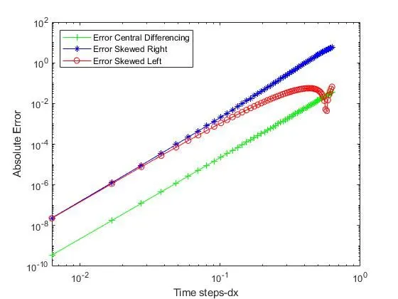
Conclusion:

Cetral differencing method has low error compared to the skewed right and skewed left scheme. But center differencing cannot be used for the boundary points, as it requies point on both the sides, hence skewed scheme is a better option for numerical approximation at the bounday points.