Week 3.5 - Deriving 4th order approximation of a 2nd order derivative using Taylor Table method

More the order of approximation, more is the accuracy. Finite difference approximation: In this approach we approximate the derivative based on values of points in the neighborhood of the point. The accuracy of a finite difference approximation
depends on the accuracy of the data points, the spacing between the point, and the specific formula used for the approximation.

Central difference: the first derivative xi is approximated by the slope of the line connecting xi and xi + 1. From p + q - 1 = 5, which are the nodes for the approximation, we get,

	f(x)	f'(x)dx	f''(x)(dx)^2	f"'(x)(dx)^3	f''''(x)(dx)^4	f'''''(x)(dx)^5
af(i-2)	a	-2a	4a/2	-8a/6	16a/24	-32a/120
bf(i-1)	b	-b	b/2	-b/6	b/24	-b/120
c	c	0	0	0	0	0
df(i+1)	d	d	d/2	d/6	d/24	d/120
ef(i+2)	e	2e	4e/2	8e/6	16e/24	32e/120
sum	0	0	1	0	0	?

Solving the Matrix, we get a = -0.0833, b = 1.3333, c = -2.500, d = 1.3333, e = -0.0833

Skewed scheme: number of nodes = p + q where p = order of derivative and q = order of approximation

For right-sided difference: number of nodes = 6

	f(x)	f'(x)dx	f''(x)(dx)^2	f"'(x)(dx)^3	f''''(x)(dx)^4	f'''''(x)(dx)^5
af(i)	a	0	0	0	0	0
bf(i+1)	b	b	b/2	b/6	b/24	b/120
c(i+2)	c	2c	4c/2	8c/6	16b/24	32c/120
df(i+3)	d	3d	9d/2	27d/6	81d/24	243d/120
ef(i+4)	e	4e	16e/2	64e/6	256e/24	1024e/120
gf(i+5)	f	5f	25f/2	125f/6	625f/24	3125f/120
sum	0	0	1	0	0	0

Solving the Matrix, we get a = 3.75, b = -12.833, c = 17.833, d = -13.00, e = 5.0833, f = -0.8333

For left-sided difference: number of nodes = 6

	f(x)	f'(x)dx	f''(x)(dx)^2	f"'(x)(dx)^3	f''''(x)(dx)^4	f'''''(x)(dx)^5
af(i-5)	a	-5a	25a/2	-125a/6	625a/24	-3125a/120
bf(i-4)	b	-4b	16b/2	-64b/6	256b/24	-1024b/120
c(i-3)	c	-3c	9c/2	-27c/6	81c/24	-243c/120
df(i-2)	d	-2b	4d/2	-8d/6	16d/24	-32d/120
ef(i-1)	e	-e	e/2	-e/6	e/24	-e/120
gf(i)	f	0	0	0	0	0
sum	0	0	1	0	0	0

Solving the Matrix, we get a = -0.8333, b = 5.0833, c = -13.00, d = 17.833, e = -12.833 , f = 3.7500

In order to prove the skewed schemes are fourth order accurate, the Taylor series expansion with the coefficients is

d²f/dx² = af(i-5) + bf(i-4) + cf(i-3) + df(i-2) + ef(i-1) + gf(i)

Substituting the value of coefficients for left skewed scheme,

0 + 0 + f”(i) (dx)² + 0 + 0 + ((3125/144) a + (256/45)b + (81/80)c + (4/45)d + e/720) f₆(i) (dx)⁶

Dividing by (dx)²

d²f/dx² = af(i-5) + bf(i-4) + cf(i-3) + df(i-2) + ef(i-1) + gf(i) /dx² = f”(i) + O(dx)⁴

Hence this represents a truncation error of fourth order due to elimination of the fourth order terms.

clear all
close all
clc

x = pi/3;
dx = linspace(pi/4000, pi/40,20);

for i = 1:length(dx)
    error_central(i) = central(x,dx(i));
    error_right(i) = skewed_right(x,dx(i));
    error_left(i) = skewed_left(x,dx(i));
    
end

figure(1)
loglog(dx, error_central, 'r-', dx, error_right, 'g-', dx, error_left, 'y-')
xlabel('Discretization of x')
ylabel('Error in approximation')
title('Error for different approximation schemes')
legend('Error Central', 'Error Right skewed scheme', 'Error left skewed scheme')

function [out] = central(x,dx)

exact_derivative = -2*exp(x)*sin(x);
%Coefficients from Taylor's Table
a = -0.0833;
b = 1.3333;
c = -2.500;
d = 1.333;
e = -0.0833;

s = (a*exp(x-2*dx)*cos(x-2*dx) + b*exp(x-dx)*cos(x-dx) + c*exp(x)*cos(x) + d*exp(x+dx)*cos(x+dx) + e*exp(x+2*dx)*cos(x+2*dx))/(dx)^2;
out = abs(s - exact_derivative);
end

function [out] = skewed_right(x,dx)

exact_derivative = -2*exp(x)*sin(x);
%Coefficients from Taylor's Table
a = 3.75;
b = -12.83333;
c = 17.8333;
d = -13.000;
e = 5.08333;
f = -0.0833;

s = (a*exp(x)*cos(x) + b*exp(x+dx)*cos(x+dx) + c*exp(x+2*dx)*cos(x+2*dx) + d*exp(x+3*dx)*cos(x+3*dx) + e*exp(x+4*dx)*cos(x+4*dx)+ f*exp(x+5*dx)*cos(x+5*dx))/(dx)^2;
out = abs(s - exact_derivative);
end

function [out] = skewed_left(x,dx)

exact_derivative = -2*exp(x)*sin(x);
%Coefficients from Taylor's Table
a = -0.0833;
b = 5.08333;
c = -13.000;
e = 17.8333;
d = -12.83333;
f = 3.75;

s = (a*exp(x)*cos(x) + b*exp(x-dx)*cos(x-dx) + c*exp(x-2*dx)*cos(x-2*dx) + d*exp(x-3*dx)*cos(x-3*dx) + e*exp(x-4*dx)*cos(x-4*dx)+ f*exp(x-5*dx)*cos(x-5*dx))/(dx)^2;
out = abs(s - exact_derivative);
end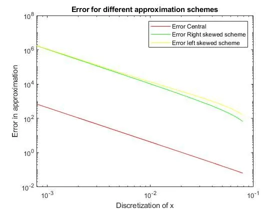

It can be seen that the error is least when it comes to centrally skewed scheme. However a skewed scheme is useful because it can predict the derivative of a function when values towards one side are known (either right or left) and does not require both. This information may be easily available which makes them more useful compared to centrally skewed scheme which requires both sides of the function value to be known.