Week 3.5 - Deriving 4th order approximation of a 2nd order derivative using Taylor Table method

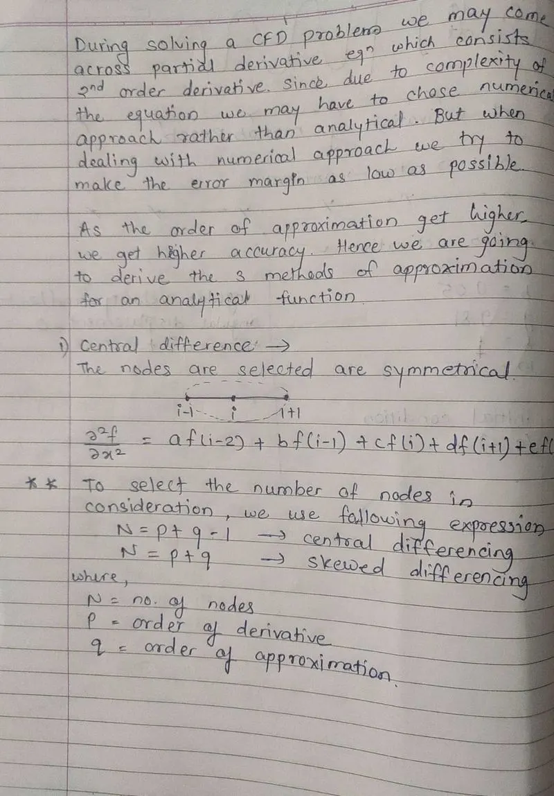
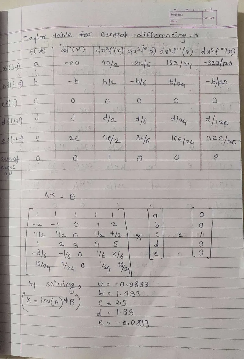
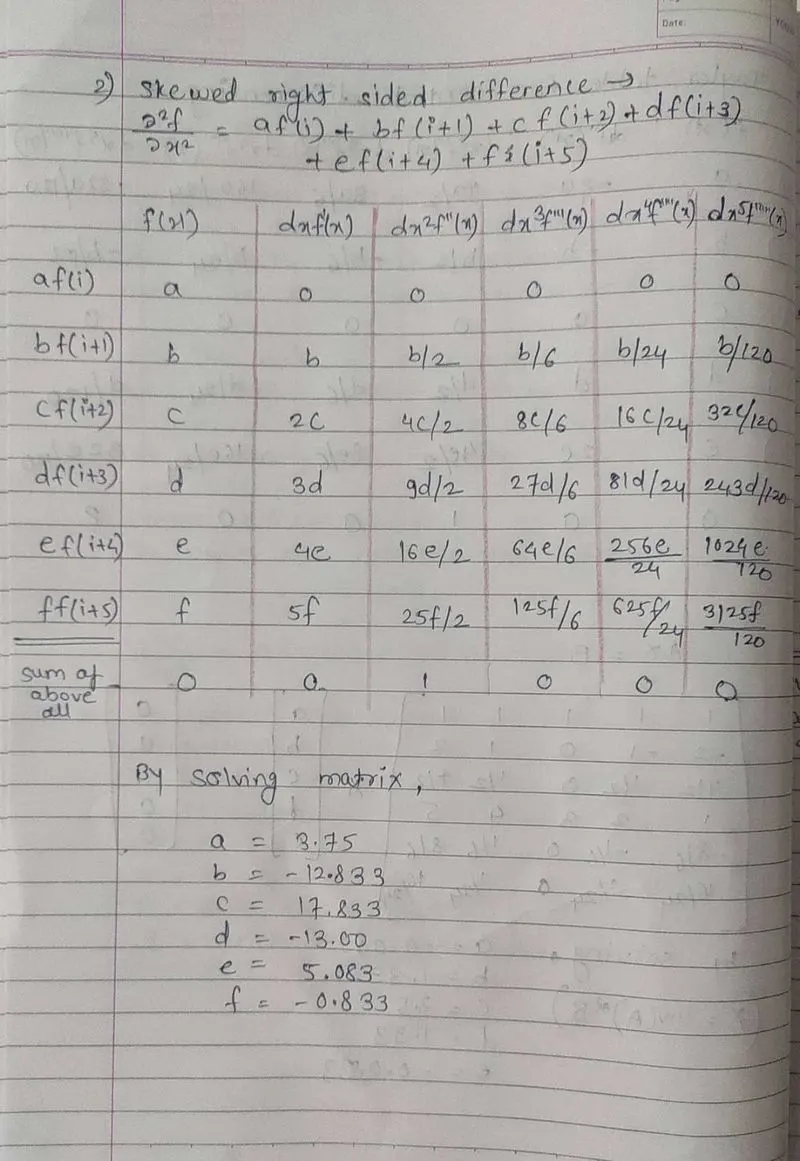
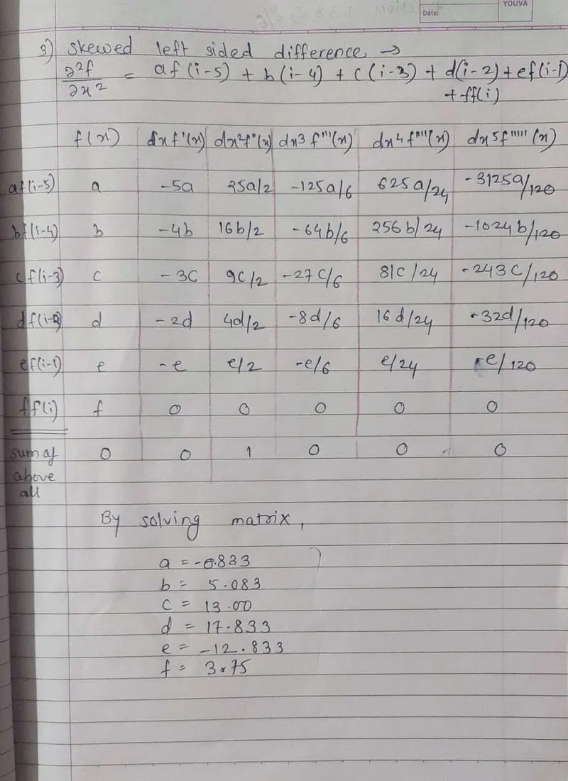
code for matlab-

clear all
close all
clc

%value of x
x=pi/3;
%range of dx
dx=linspace(pi/6,pi/700,20);
%for loop
for i=1:length(dx)
Central_differencing(i)=fourth_order_Central_differencing(x,dx(i));
right_sided_skew(i)=fourth_order_right_sided_skew(x,dx(i));
left_sided_skew(i)=fourth_order_left_sided_skew(x,dx(i));
end

%plotting
figure(1)
loglog(dx,Central_differencing,'g')
hold on
loglog(dx,right_sided_skew,'r')
hold on
loglog(dx,left_sided_skew,'b')
xlabel('range of dx')
ylabel('error')
title('range of dx vs error')
legend('central differncing','skewed right sided difference','skewed left sided difference','location','northwest')

##function code for Central_differencing

function error_Central_differencing=fourth_order_Central_differencing(x,dx)

%analytical function = exp(x)*cos(x)

%analytical derivative
%f''(x)= -2*exp(x)*sin(x)
analytical_derivative = -2*exp(x)*sin(x);
%numerical derivative
xm2 = x-(2*dx);
xm1 = x-(1*dx);
xp1 = x+(1*dx);
xp2 = x+(2*dx);

f_xm2 = exp(xm2)*cos(xm2);
f_xm1 = exp(xm1)*cos(xm1);
f_x = exp(x)*cos(x);
f_xp1 = exp(xp1)*cos(xp1);
f_xp2 = exp(xp2)*cos(xp2);

Central_differencing= (-0.08333333333333333333333*f_xm2 + 1.33333333333333333333333333*f_xm1 -2.5*f_x + 1.33333333333333333333333*f_xp1 - 0.083333333333333333333*f_xp2)/(dx^2);

%error
error_Central_differencing= abs(Central_differencing - analytical_derivative);
end

##function code for right_sided_skew

function error_right_sided_skew=fourth_order_right_sided_skew(x,dx)

%analytical function = exp(x)*cos(x)

%analytical derivative
%f''(x)= -2*exp(x)*sin(x)
analytical_derivative = -2*exp(x)*sin(x);

xp1 = x+(1*dx);
xp2 = x+(2*dx);
xp3 = x+(3*dx);
xp4 = x+(4*dx);
xp5 = x+(5*dx);

f_x = exp(x)*cos(x);
f_xp1 = exp(xp1)*cos(xp1);
f_xp2 = exp(xp2)*cos(xp2);
f_xp3 = exp(xp3)*cos(xp3);
f_xp4 = exp(xp4)*cos(xp4);
f_xp5 = exp(xp5)*cos(xp5);

right_sided_skew = (3.75*f_x + (-12.8333333333333333333333333)*f_xp1 + 17.8333333333333333333333333333333*f_xp2 -13.0*f_xp3 + 5.08333333333333333333333333333333*f_xp4 -0.83333333333333333333333333333333*f_xp5)/(dx^2);

%numerical derivative
% right_sided_skew = (((3.7500)*((exp(x))*(cos(x))))-((12.8333)*((exp(x+dx))*(cos(x+dx))))+(17.8333)*((exp(x+(2*dx)))*(cos(x+(2*dx)))))-((13.0)*((exp(x+(3*dx)))*(cos(x+(3*dx)))))+((5.0833)*((exp(x+(4*dx)))*(cos(x+(4*dx)))))-((0.8333)*((exp(x+(5*dx)))*(cos(x+(5*dx)))))/(dx^2);

%error
error_right_sided_skew= abs(right_sided_skew - analytical_derivative);
end

##function code for left_sided_skew

function error_left_sided_skew=fourth_order_left_sided_skew(x,dx)

%analytical function = exp(x)*cos(x)

%analytical derivative
%f''(x)= -2*exp(x)*sin(x)
analytical_derivative = -2*exp(x)*sin(x);

xp1 = x-(1*dx);
xp2 = x-(2*dx);
xp3 = x-(3*dx);
xp4 = x-(4*dx);
xp5 = x-(5*dx);

f_x = exp(x)*cos(x);
f_xp1 = exp(xp1)*cos(xp1);
f_xp2 = exp(xp2)*cos(xp2);
f_xp3 = exp(xp3)*cos(xp3);
f_xp4 = exp(xp4)*cos(xp4);
f_xp5 = exp(xp5)*cos(xp5);

%numerical derivative
left_sided_skew = ((-0.83333333333333333)*f_xp5 + 5.08333333333333333 *f_xp4 - 13.0 *f_xp3 + 17.833333333333333333*f_xp2 -(12.83333333333333333)*f_xp1 + 3.7500 *f_x)/(dx^2);

%error
error_left_sided_skew= abs(left_sided_skew - analytical_derivative);
end

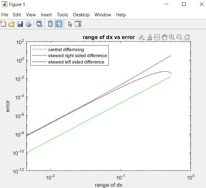
Result-

Conclusion-

1.Central differencing method has less error than other two methods.

2.If we don't have sufficient information on both side of point then we need to use skewed scheme.

3. CDS can not be employed at the boundary nodes due to unavailability of right and left nodes at the same time. In such cases skewed differencing scheme is useful.