Week 3.5 - Deriving 4th order approximation of a 2nd order derivative using Taylor Table method

The given function in the question is `y=e^x*cos(x)` --- Equation (1)

In the above expression, both the terms on the RHS are functions of x and differentiable with x. For differentiating the above expression we need to apply the product rule.

`(dy)/dx =((d(e^x.cos(x)))/dx)`

`(dy)/dx=e^x*(d(cos(x)))/dx+cos(x)*(d(e^x))/dx`

`(dy)/dx=-e^x*sin(x)+e^x*cos(x) =e^x*(cos(x)-sin(x))`--- Equation (2)

`(d^2y)/dx^2=-2e^x*Sinx`--- Equation(2a)

Equation(2a) is the analytical solution (second derivative) of equation (1)

Numerical derivative using Taylor table method:

1. Central difference method
   

The derivation of the equation for evaluating the second-order numerical derivative with the fourth-order central difference approximation method is as given below.

For the central differencing scheme, the number of nodes in the stencils is found by the following thumb rule,

n=p+q-1

Where,

n= number of nodes in the stencil

p=order of accuracy/approximation

q=order on the numerical derivative

For the present problem statement, p=4, q=2. Hence, n=5.

We will be using the Taylor table method, and the general equation for evaluating the second-order derivative using the fourth-order accurate central difference method is as follows

`Deltax^2*f''(x)= Deltax^2*(d^2y)/(dx^2)=a*f(x)+b*f(x+Deltax)+c*f(x+2Deltax)+d*f(x-Deltax)+e*f(x-2Deltax)`--- Equation(3)

`f''(x)= (Deltax^2*(d^2y)/(dx^2)=a*f(x)+b*f(x+Deltax)+c*f(x+2Deltax)+d*f(x-Deltax)+e*f(x-2Deltax))/(Deltax^2)`--- Equation(3a)

Table-1:Taylor table for fourth-order accurate central difference method

	`f(x)`	`Deltax*f'(x)`	`Deltax^2*f^((2))(x)`	`Deltax^3*f^((3))(x)`	`Deltax^4*f^((4))(x)`
`a.f(x)`	a	0	0	0	0
`b*f(x+DeltaX)`	`b`	`b`	`b/2`	`b/6`	`b/24`
`c*f(x+2DeltaX)`	`c`	`2c`	`(4c)/2`	`(8c)/6`	`(16c)/24`
`d*f(x-DeltaX)`	`d`	`-d`	`d/2`	`-d/6`	`d/24`
`e*f(x-2DeltaX)`	`e`	`-2e`	`(4e)/2`	`(-8e)/6`	`(16e)/24`
Summation of coefficients	0	0	1	0	0

By solving equation(3) we will be able to determine the second order numeraical derivative of the given function.However, to solve this equation(3) , we need to determine the values of these coefficients (a,b,c,d, and e) mentioned in Table-1.

`a+b+c+d+e=0`---Equation(4)

`b+2c-d-2e=0`---Equation(5)

`(b+4c+d+4e)/2=1`--- Equation(6)

`(b+8c-d-8e)/6=0`---Equation(7)

`(b+16c+d+16e)/24=0`---Equation(8)

We can determine the values of this co-efficient by solving the five equations (equation(4) to equation(8)) for five unknowns. We got these by equating the LHS of equation(3) and the summation of coefficients from the Taylor table (Table-1).

In the LHS of equation (3) we can see that there is only one term i.e., `Deltax^2*f^((2))(x)`; Hence, the summation of coefficients of `Deltax^2*f^((2))(x)` in Taylor table are equated to 1 and rest all summations are equated to 0.

These equations starting from equations (4) to equation(8) are represented below in the form of a matrix. As mentioned in the question, we need to solve these equations using the matrix inversion method in MatLab to get these coefficients.

`[[1,1,1,1,1 ],[0,1,2,-1,-2],[0,1/2,4/2,1/2,4/2],[0,1/6,8/6,-1/6,-8/6],[0,1/24,16/24,1/24,16/24]][[a],[b],[c],[d],[e]]=[[0],[0],[1],[0],[0]]`--- Equation (9)

The above matrix is of the form `AX=B`--- Equation(10)

where `A=[[1,1,1,1,1 ],[0,1,2,-1,-2],[0,1/2,4/2,1/2,4/2],[0,1/6,8/6,-1/6,-8/6],[0,1/24,16/24,1/24,16/24]]` ; `X=[[a],[b],[c],[d],[e]]`; and `B=[[0],[0],[1],[0],[0]]`

We need to find the terms in X. By multiplying both sides of equation (10) by `A^-1` we get

`A^-1*A*X=A^-1*B`

Where `A^-1` is the inverse of matrix `A`. The inverse of a matrix is a matrix that multiplied by the original matrix results in the identity matrix, regardless of the order of the matrix multiplication.

`X=A^-1*B`---Equation (11)

A Matlab function is written to determine the elements (a,b,c,d,e) of Matrix `X`. Further, these elements (a,b,c,d,e) are subsituted back in equation (3a) to determine the fourth order accurate second order derivative for a given `DeltaX`

After determining the numerical derivative we can determine the error associated with this method by finding the absolute difference between the analytical derivative and numerical derivative. The script of the Matlab function written for determining the fourth-order accurate second-order derivative using the central differencing method is given below:

function out=taylor_table_fourth_CD_func(x, dx)
% analytical function = e^x*cos(x)
% second order analytical derivative = -2e^x*sin(x)
%Analytical derivative of the given function
analytical_derivative =-2*exp(x)*sin(x);

%%
%numerical derivative: fourth order acurate central differencing 
%second order derivative using taylor table method 
%Delta_x^2*f''(x)=(a*f(x))+(b*f(x+Delta_x))+(c*f(x+2*Delta_x))+(d*f(x-Delta_x))+(e*f(x-2*Delta_x))

%Summation of coefficients of terms in Taylor series. It is a column
%matrix which is represented by B
B=[0;0;1;0;0];

%Constants in the Taylor series expansion which is represented by A.
A=[1,1,1,1,1 ;0,1,2,-1,-2; 0,1/2,4/2,1/2,4/2; 0,1/6,8/6,-1/6,-8/6; 0,1/24,16/24,1/24,16/24];

%Following is the array of multipliers that needs to be determined to
%evaluate the numerical derivative The column matrix of multipliers is
%represented by X.
%X=[a, b, c, d, e];

%inverse of matrix A is found by the following command.
A_inverse=inv(A);

%The values in the column matrix X is determined by the following command
X=A_inverse*B;

%Just for ease of understanding and creating the relationship between the
%explanantion in the report and the code written here, the elements of the
%matrix are assigned to variables a, b, c, d, and e
a=X(1);b=X(2); c=X(3); d=X(4); e=X(5);

fourth_order_CD =((a*exp(x)*cos(x))+(b*exp(x+dx)*cos(x+dx))+(c*exp(x+2*dx)*cos(x+2*dx))+(d*exp(x-dx)*cos(x-dx))+(e*exp(x-2*dx)*cos(x-2*dx)))/(dx^2);

%%
%Calculating the error.
%Calculating fourth order error
out=abs(fourth_order_CD-analytical_derivative);

2. Skewed right-sided difference method

The derivation of the equation for evaluating the second-order numerical derivative with the fourth-order skewed right-sided difference method is as given below.

For a one-sided differencing scheme, the number of nodes in the stencils is found by the following thumb rule,

n=p+q

Where,

n= number of nodes in the stencil

p=order of accuracy/approximation

q=order on the numerical derivative

For the present problem statement, p=4, q=2. Hence, n=6.

We will be using the Taylor table method, and the general equation for evaluating the second-order derivative using the fourth-order accurate skewed right-sided difference method is as follows

`Deltax^2*f''(x)= Deltax^2*(d^2y)/(dx^2)=a_1*f(x)+b_1*f(x+Deltax)+c_1*f(x+2Deltax)+d_1*f(x+3Deltax)+e_1*f(x+4Deltax)+g_1*f(x+5DeltaX)`--- Equation(12)

`f''(x)= Deltax^2*(d^2y)/(dx^2)=a_1*f(x)+b_1*f(x+Deltax)+c_1*f(x+2Deltax)+d_1*f(x+3Deltax)+e_1*f(x+4Deltax)+g_1*f(x+5DeltaX)/(Deltax^2)`--- Equation(12a)

Table-2:Taylor table for fourth-order accurate skewed right-sided central difference method

	`f(x)`	`Deltax*f'(x)`	`Deltax^2*f^((2))(x)`	`Deltax^3*f^((3))(x)`	`Deltax^4*f^((4))(x)`	`Deltax^5*f^((5))(x)`
`a_1.f(x)`	`a_1`	0	0	0	0	0
`b_1*f(x+DeltaX)`	`b_1`	`b_1`	`b_1/2`	`b_1/6`	`b_1/24`	`b_1/120`
`c_1*f(x+2DeltaX)`	`c_1`	`2c_1`	`(4c_1)/2`	`(8c_1)/6`	`(16c_1)/24`	`(32c_1)/120`
`d_1*f(x+3DeltaX)`	`d_1`	`3d_1`	`(9d_1)/2`	`(27d_1)/6`	`(81d_1)/24`	`(243d_1)/120`
`e_1*f(x+4DeltaX)`	`e_1`	`4e_1`	`(16e_1)/2`	`(64e_1)/6`	`(256e_1)/24`	`(1024e_1)/120`
`g_1*f(x+5DeltaX)`	`g_1`	`5g_1`	`(25g_1)/2`	`(125g_1)/6`	`(625g_1)/24`	`(3125g_1)/120`
Summation of coefficients	0	0	1	0	0	0

By solving equation(12) we will be able to determine the second order numeraical derivative of the given function.However, to solve this equation, we need to determine the values of these coefficients (`a_1,b_1, c_1,d_1, e_1, g_1`) mentioned in Table-2.

`a_1+b_1+c_1+d_1+e_1+g_1=0`---Equation(13)

`b_1+2c_1+3d_1+4e_1+5g_1=0`---Equation(14)

`(b_1+4c_1+9d_1+16e_1+25g_1)/2=1`--- Equation(15)

`(b_1+8c_1+27d_1+64e_1+125g_1)/6=0`---Equation(16)

`(b_1+16c_1+81d_1+256e_1+625g_1)/24=0`---Equation(17)

`(b_1+32c_1+243d_1+1024e_1+3125g_1)/120=0`---Equation(18)

We can determine the values of this co-efficient by solving the six equations (equation(13) to equation(18)) for six unknowns. We got these by equating the LHS of equation(12) and the summation of coefficients from the Taylor table (Table-2).

In the LHS of equation (12) we can see that there is only one term i.e., `Deltax^2*f^((2))(x)`; Hence, the summation of coefficients of `Deltax^2*f^((2))(x)` in Taylor table are equated to 1 and rest all summations are equated to 0.

These equations starting from equations (13) to equation(18) are represented below in the form of a matrix. As mentioned in the question, we need to solve these equations using the matrix inversion method in MatLab to get these coefficients.

`[[1,1,1,1,1,1],[0,1,2,3,4,5],[0,1/2,4/2,9/2,16/2,25/2],[0,1/6,8/6,27/6,64/6,125/6],[0,1/24,16/24,81/24,256/24,625/24],[0,1/120,32/120,243/120,1024/120,3125/120]][[a_1],[b_1],[c_1],[d_1],[e_1],[g_1]]=[[0],[0],[1],[0],[0],[0]]`--- Equation (19)

The above matrix is of the form `A_1X_1=B_1`--- Equation(20)

where `A_1=[[1,1,1,1,1,1],[0,1,2,3,4,5],[0,1/2,4/2,9/2,16/2,25/2],[0,1/6,8/6,27/6,64/6,125/6],[0,1/24,16/24,81/24,256/24,625/24],[0,1/120,32/120,243/120,1024/120,3125/120]]` ; `X_1=[[a_1],[b_1],[c_1],[d_1],[e_1],[g_1]]`; and `B_1=[[0],[0],[1],[0],[0],[0]]`

We need to find the terms in `X_1`. By multiplying both sides of equation (10) by `A_1^-1` we get

`A_1^-1*A_1*X_1=A_1^-1*B_1`

Where `A_1^-1` is the inverse of matrix `A_1`. The inverse of a matrix is a matrix that multiplied by the original matrix results in the identity matrix, regardless of the order of the matrix multiplication.

`X_1=A_1^-1*B_1`---Equation (21)

A Matlab function is written to determine the elements (a,b,c,d,e and g) of Matrix `X_1`. Further, these elements (`a_1,b_1, c_1,d_1, e_1, g_1`) are subsituted back in equation (12a) to determine the fourth order accurate second order derivative for a given `DeltaX`

After determining the numerical derivative we can determine the error associated with the skewed right-sided difference method by finding the absolute difference between the analytical derivative and numerical derivative. The script of the Matlab function written for determining the fourth-order accurate second-order derivative using skewed right-sided difference method is given below:

function out=taylor_table_fourth_RD_func(x, dx)
% analytical function = e^x*cos(x)
% second order analytical derivative = -2e^x*sin(x)
%Analytical derivative of the given function
analytical_derivative =-2*exp(x)*sin(x);

%%
%numerical derivative: fourth order acurate central differencing 
%second order derivative using taylor table method 
%`Deltax^2*f''(x)= Deltax^2*(d^2y)/(dx^2)=a_1*f(x)+b_1*f(x+Deltax)+c_1*f(x+2Deltax)+d_1*f(x+3Deltax)+e_1*f(x+4Deltax)+g_1*f(x+5DeltaX)`

%Summation of coefficients of terms in Taylor series. It is a column
%matrix which is represented by B
B1=[0;0;1;0;0;0];

%Constants in the Taylor series expansion which is represented by A.
A1=[1,1,1,1,1,1;0,1,2,3,4,5;0,1/2,4/2,9/2,16/2,25/2;0,1/6,8/6,27/6,64/6,125/6;0,1/24,16/24,81/24,256/24,625/24;0,1/120,32/120,243/120,1024/120,3125/120];
%Following is the array of multipliers that needs to be determined to
%evaluate the numerical derivative The column matrix of multipliers is
%represented by X.
%X=[a, b, c, d, e,g];

%inverse of matrix A1 is found by the following command.
A1_inverse=inv(A1);

%The values in the column matrix X1 is determined by the following command
X1=A1_inverse*B1;

%Just for ease of understanding and creating the relationship between the
%explanantion in the report and the code written here, the elements of the
%matrix are assigned to variables a, b, c, d, and e
a1=X1(1);b1=X1(2); c1=X1(3); d1=X1(4); e1=X1(5);g1=X1(6);

fourth_order_RD =((a1*exp(x)*cos(x))+(b1*exp(x+dx)*cos(x+dx))+(c1*exp(x+2*dx)*cos(x+2*dx))+(d1*exp(x+3*dx)*cos(x+3*dx))+(e1*exp(x+4*dx)*cos(x+4*dx))+(g1*exp(x+5*dx)*cos(x+5*dx)))/(dx^2);

%%
%Calculating the error.
%Calculating fourth order error
out=abs(fourth_order_RD-analytical_derivative);

3. Skewed Left-sided difference method

The derivation of the equation for evaluating the second-order numerical derivative with the fourth-order skewed left-sided difference method is as given below.

For the one-sided differencing scheme, the number of nodes in the stencils is found by the following thumb rule,

n=p+q

Where,

n= number of nodes in the stencil

p=order of accuracy/approximation

q=order on the numerical derivative

For the present problem statement, p=4, q=2. Hence, n=6.

We will be using the Taylor table method, and the general equation for evaluating the second-order derivative using the fourth-order accurate skewed left-sided difference method is as follows

`Deltax^2*f''(x)= Deltax^2*(d^2y)/(dx^2)=a_2*f(x)+b_2*f(x-Deltax)+c_2*f(x-2Deltax)+d_2*f(x-3Deltax)+e_2*f(x-4Deltax)+g_2*f(x-5DeltaX)`--- Equation(22)

`f''(x)= Deltax^2*(d^2y)/(dx^2)=a_2*f(x)+b_2*f(x-Deltax)+c_2*f(x-2Deltax)+d_2*f(x-3Deltax)+e_2*f(x-4Deltax)+g_2*f(x-5DeltaX)/(Deltax^2)`--- Equation(22a)

Table-3:Taylor table for fourth-order accurate skewed right-sided central difference method

	`f(x)`	`Deltax*f'(x)`	`Deltax^2*f^((2))(x)`	`Deltax^3*f^((3))(x)`	`Deltax^4*f^((4))(x)`	`Deltax^5*f^((5))(x)`
`a_2.f(x)`	`a_2`	0	0	0	0	0
`b_2*f(x-DeltaX)`	`b_2`	`-b_2`	`b_2/2`	`-b_2/6`	`b_2/24`	`-b_2/120`
`c_2*f(x-2DeltaX)`	`c_2`	`-2c_2`	`(4c_2)/2`	`-(8c_2)/6`	`(16c_2)/24`	`-(32c_2)/120`
`d_2*f(x-3DeltaX)`	`d_2`	`-3d_2`	`(9d_2)/2`	`-(27d_2)/6`	`(81d_2)/24`	`-(243d_2)/120`
`e_2*f(x-4DeltaX)`	`e_2`	`-4e_2`	`(16e_2)/2`	`-(64e_2)/6`	`(256e_2)/24`	`-(1024e_2)/120`
`g_2*f(x-5DeltaX)`	`g_2`	`-5g_2`	`(25g_2)/2`	`-(125g_2)/6`	`(625g_2)/24`	`-(3125g_2)/120`
Summation of coefficients	0	0	1	0	0	0

By solving equation(22) we will be able to determine the second order numeraical derivative of the given function.However, to solve this equation, we need to determine the values of these coefficients (`a_2,b_2, c_2,d_2, e_2, g_2`) mentioned in Table-3.

`a_2+b_2+c_2+d_2+e_2+g_2=0`---Equation(23)

`-b_2-2c_2-3d_2-4e_2-5g_2=0`---Equation(24)

`(b_2+4c_2+9d_2+16e_2+25g_2)/2=1`--- Equation(25)

`(-b_2-8c_2-27d_2-64e_2-125g_2)/6=0`---Equation(26)

`(b_2+16c_2+81d_2+256e_2+625g_2)/24=0`---Equation(27)

`(-b_2-32c_2-243d_2-1024e_2-3125g_2)/120=0`---Equation(28)

We can determine the values of this co-efficient by solving the six equations (equation(23) to equation(28)) for six unknowns. We got these by equating the LHS of equation(22) and the summation of coefficients from the Taylor table (Table-3).

In the LHS of equation (22) we can see that there is only one term i.e., `Deltax^2*f^((2))(x)`; Hence, the summation of coefficients of `Deltax^2*f^((2))(x)` in Taylor table are equated to 1 and rest all summations are equated to 0.

These equations starting from equations (23) to equation(28) are represented below in the form of a matrix. As mentioned in the question, we need to solve these equations using the matrix inversion method in MatLab to get these coefficients.

`[[1,1,1,1,1,1],[0,-1,-2,-3,-4,-5],[0,1/2,4/2,9/2,16/2,25/2],[0,-1/6,-8/6,-27/6,-64/6,-125/6],[0,1/24,16/24,81/24,256/24,625/24],[0,-1/120,-32/120,-243/120,-1024/120,-3125/120]][[a_2],[b_2],[c_2],[d_2],[e_2],[g_2]]=[[0],[0],[1],[0],[0],[0]]`--- Equation (29)

The above matrix is of the form `A_2X_2=B_2`--- Equation(30)

where `A_2=[[1,1,1,1,1,1],[0,-1,-2,-3,-4,-5],[0,1/2,4/2,9/2,16/2,25/2],[0,-1/6,-8/6,-27/6,-64/6,-125/6],[0,1/24,16/24,81/24,256/24,625/24],[0,-1/120,-32/120,-243/120,-1024/120,-3125/120]]` ; `X_2=[[a_2],[b_2],[c_2],[d_2],[e_2],[g_2]]`; and `B_2=[[0],[0],[1],[0],[0],[0]]`

We need to find the terms in `X_2`. By multiplying both sides of equation (30) by `A_2^-1` we get

`A_2^-1*A_2*X_2=A_2^-1*B_2`

Where `A_2^-1` is the inverse of matrix `A_2`. The inverse of a matrix is a matrix that multiplied by the original matrix results in the identity matrix, regardless of the order of the matrix multiplication.

`X_2=A_2^-1*B_2`---Equation (31)

A Matlab function is written to determine the elements (`a_2,b_2, c_2,d_2, e_2, g_2`) of Matrix `X_2`. Further, these elements (`a_2,b_2, c_2,d_2, e_2, g_2`) are subsituted back in equation (22a) to determine the fourth order accurate second order derivative for a given `DeltaX`

After determining the numerical derivative we can determine the error associated with the skewed right-sided difference method by finding the absolute difference between the analytical derivative and numerical derivative. The script of the Matlab function written for determining the fourth-order accurate second-order derivative using skewed left-sided difference method is given below:

function out=taylor_table_fourth_LD_func(x, dx)
% analytical function = e^x*cos(x)
% second order analytical derivative = -2e^x*sin(x)
%Analytical derivative of the given function
analytical_derivative =-2*exp(x)*sin(x);

%%
%numerical derivative: fourth order acurate central differencing 
%second order derivative using taylor table method 
%`Deltax^2*f''(x)= Deltax^2*(d^2y)/(dx^2)=a_2*f(x)+b_2*f(x-Deltax)+c_2*f(x-2Deltax)+d_2*f(x-3Deltax)+e_2*f(x-4Deltax)+g_2*f(x-5DeltaX)`

%Summation of coefficients of terms in Taylor series. It is a column
%matrix which is represented by B
B2=[0;0;1;0;0;0];

%Constants in the Taylor series expansion which is represented by A.
A2=[1,1,1,1,1,1;0,-1,-2,-3,-4,-5;0,1/2,4/2,9/2,16/2,25/2;0,-1/6,-8/6,-27/6,-64/6,-125/6;0,1/24,16/24,81/24,256/24,625/24;0,-1/120,-32/120,-243/120,-1024/120,-3125/120];
%Following is the array of multipliers that needs to be determined to
%evaluate the numerical derivative The column matrix of multipliers is
%represented by X.
%X=[a, b, c, d, e,g];

%inverse of matrix A1 is found by the following command.
A2_inverse=inv(A2);

%The values in the column matrix X1 is determined by the following command
X2=A2_inverse*B2;

%Just for ease of understanding and creating the relationship between the
%explanantion in the report and the code written here, the elements of the
%matrix are assigned to variables a, b, c, d, and e
a2=X2(1);b2=X2(2); c2=X2(3); d2=X2(4); e2=X2(5);g2=X2(6);

fourth_order_LD =((a2*exp(x)*cos(x))+(b2*exp(x-dx)*cos(x-dx))+(c2*exp(x-2*dx)*cos(x-2*dx))+(d2*exp(x-3*dx)*cos(x-3*dx))+(e2*exp(x-4*dx)*cos(x-4*dx))+(g2*exp(x-5*dx)*cos(x-5*dx)))/(dx^2);

%%
%Calculating the error.
%Calculating fourth order error
out=abs(fourth_order_LD-analytical_derivative);

Explanation of the main program is as follows:

Finally, the above-explained functions are called in the main program to determine the associated errors with these approximation methods over a range of dx values.

The range of dx across which the error needs to be evaluated is as given below.

dx = [pi/4000,pi/40,50]

The error is determined for a total of 50 dx values with all three schemes (central difference, skewed right-sided, and skewed left-sided)

The value of x and dx are declared in the main program/script. Further, the functions written to calculate the errors associated with different schemes are called in the 'for loop'. In the for loop three arrays are generated; one array for every approximation method. The array will contain the list of errors calculated for every dx value.

All the three arrays are plotted against the dx values to understand:

• which approximation method results in the least error and
• change in error with a change in dx value

clear all
close all
clc

%Defining the value of x
x=pi/3;
%defining the list of dx values
dx=linspace(pi/4000, pi/40, 50);

%%
%loop is used to call the functions multiple times and evaluate the
%numerical derivatives by using different approximation methods. Also,
%these funcions will evaluate the error associated with respective approximation method  
for i=1:length(dx)
    left_difference_error(i)=taylor_table_fourth_LD_func(x,dx(i));
    central_difference_error(i)=taylor_table_fourth_CD_func(x,dx(i));
    right_difference_error(i)=taylor_table_fourth_RD_func(x,dx(i));
end

%%
%Plotting the error against dx values on logarithmic scale.
figure(2);
%plotting the absolute order error
loglog(dx, left_difference_error);
hold on
loglog(dx, central_difference_error,'r');
hold on
loglog(dx, right_difference_error,'k');

%Displaying the grid in the log-log plot
grid on;

%Defining the legends of the curves on the plot
legend('left difference error','central difference error','right difference error','Location','northwest')

%Defining the Label of x-axis and y-axis
xlabel('value of dx (in log_1_0)')
ylabel('Truncation error (in log_1_0)')

The output of the main program is shown below

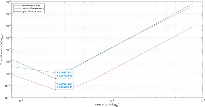
From the output is can be observed that the error associated with the central difference scheme is always smaller in comparison with the skewed right side and skewed left side difference schemes. From the graph, it can be observed that there exists one dx value i.e., 0.00237 where the error is minimum for all three schemes.

As we know that in central difference scheme the stencil is on both the side of the x. Whereas in skewed schemes, the stencil is either on the left side of the x or on the right side of the x. Skewed schemes are helpful in those situations where the x is at boundary and stencil can be taken only on one side.