Week 2 Railwheel and Track

Objective:

To perform a static structural analysis on a rail wheel and track setup and simulating the setup for the lifecycles and stress, strain and deformation observed on wheel when running on the track caused by the forces acting on the wheel.

Setup:

1. Open Ansys and select Static Structural from the toolbox.
2. Rename the Project to Rail_Wheel_Track.
   
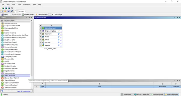
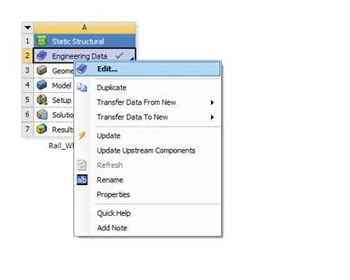
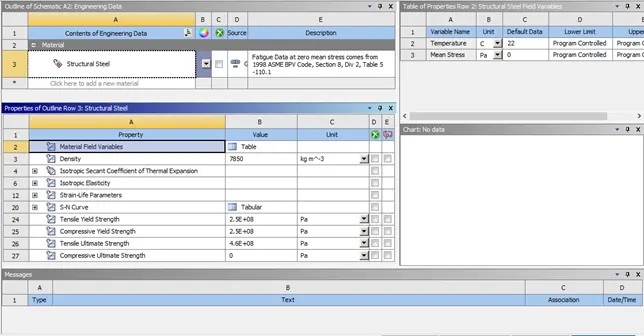
3. Right Click on Engineering Data and click on edit to select the material required for the analysis.
   
4. In this case, Structural Steel material is used for the analysis.
   
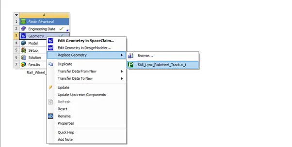
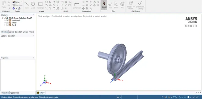
5. Import the model and open in SpaceClaim.
   
   
   
   
   
   
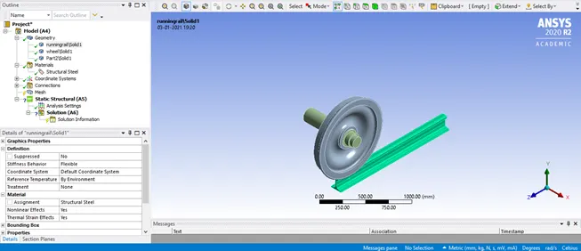
6. Open the model in Mechanical model
7. Check if all the mentioned parts are assigned with the same material i.e. Structural Steel
   
   
8. Under Connections, defaults contacts are established between the parts. Rename the contacts by definition.
   
   
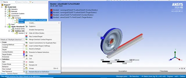
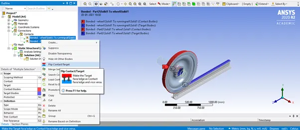
9. Flip the contact and target bodies by using the Flip Contact/Target option.
   
   
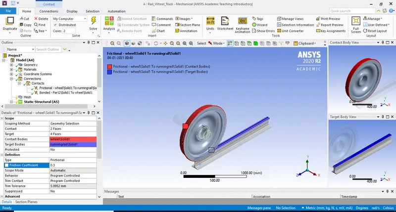
10. Provide a frictional contact between the rail wheel and track having a frictional coefficient value of 0.3.
    
    
    
    
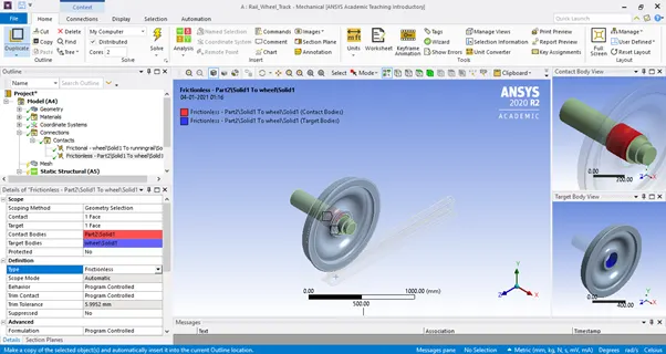
11. Provide a frictionless contact between the solid part and the wheel.
    
    
12. After assigning the respective parameters, joint loads have to be assigned to the system to run the simulation process and to evaluate the results.
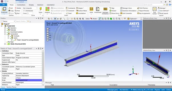
13. Apply a fixed Joint to the track for its non – moment and easy translation of the wheel on the track.
    
    
    
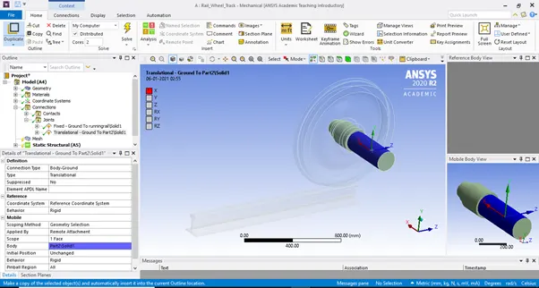
14. A translational Joint is applied on the shaft. As observed, the shaft is attached to the wheel and hence when the forces act on the shaft those forces will be translational to the wheel.
    
    
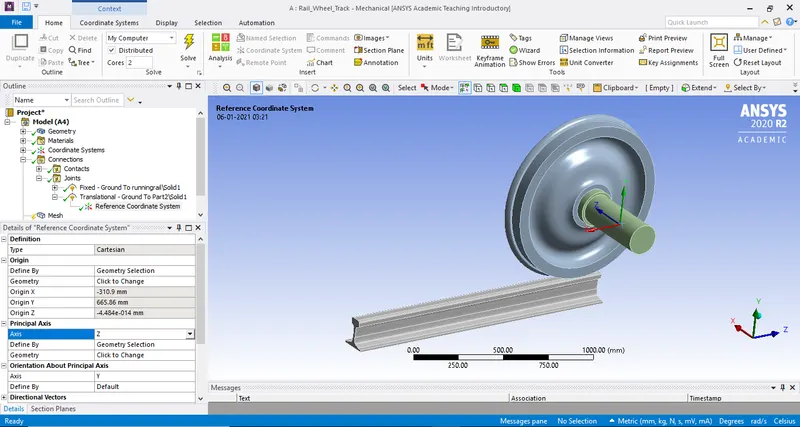
15. Check the direction of the translation joint acting. If any need to the change the direction, change the Principal Axis.
    
    
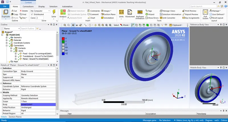
16. Finally, a planar Joint is provided to the wheel.
    
    
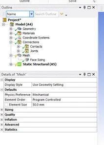
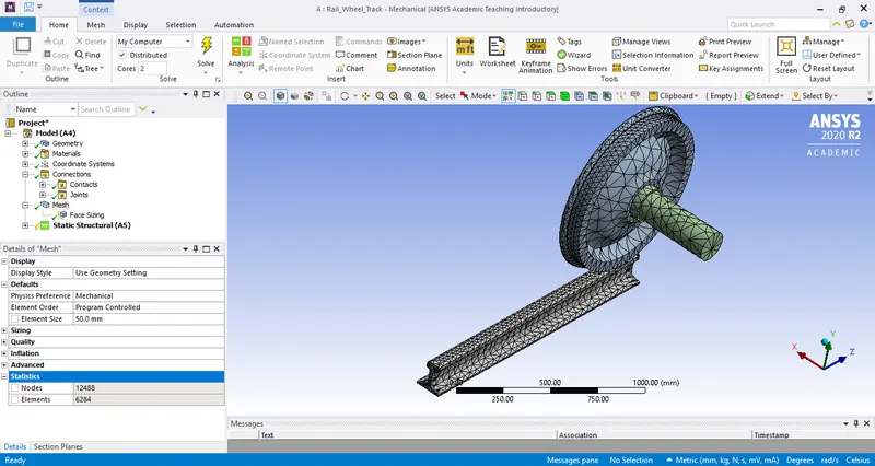
17. Generate a mesh with overall mesh size of 50mm.
    
    
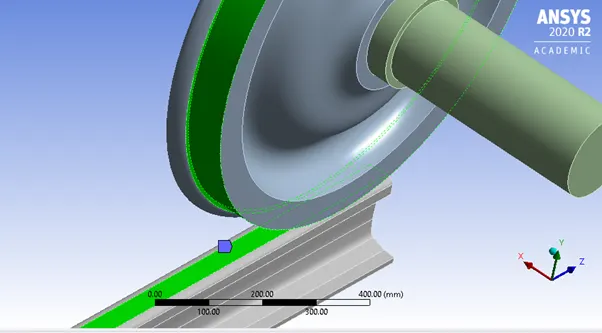
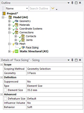
18. Select the faces (3 faces) that are in contact and apply a mesh sizing feature having a mesh size of 35mm.
    
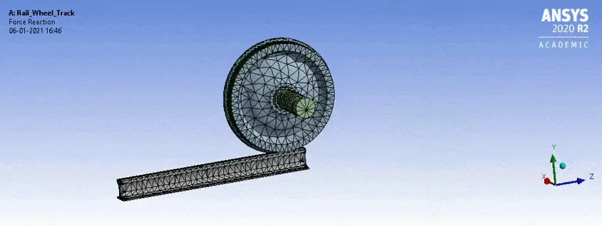
19. The generated mesh will be observed as follows.
    
    
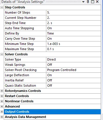
20. In the analysis settings, give appropriate parameters to the setup and define joint loads that will be applied on the geometry setup.
    
    
    
    
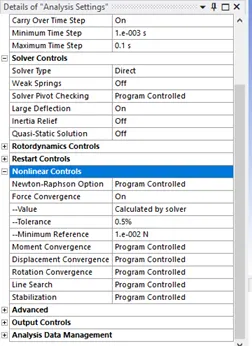
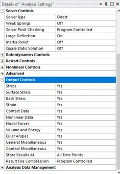
21. Switch on Force Convergence and change all the output controls to “Yes”.
    
    
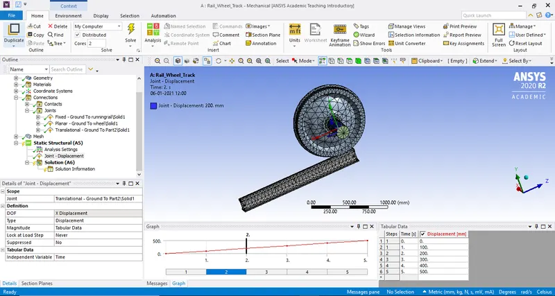
22. After the analysis parameters are given, Apply a Displacement joint to the shaft.
    
    
    
    
23. Apply a bearing load of 100000N and 500000N accordingly.
    
    
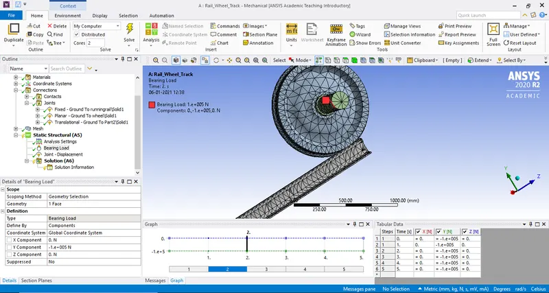
24. The setup is now complete. Solve and evaluate the necessary results.
    
    
    
    
    
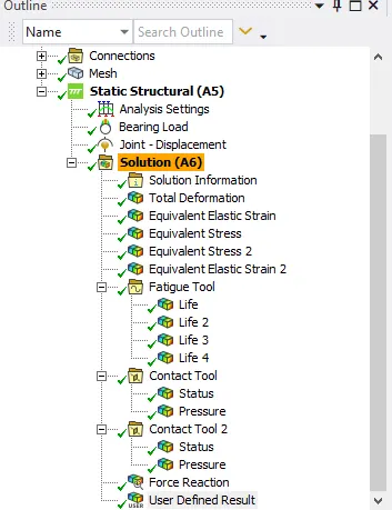
25. RESULT:
    
    

    1. Case 1: a. Bearing Load of 100KN applied.
       
       

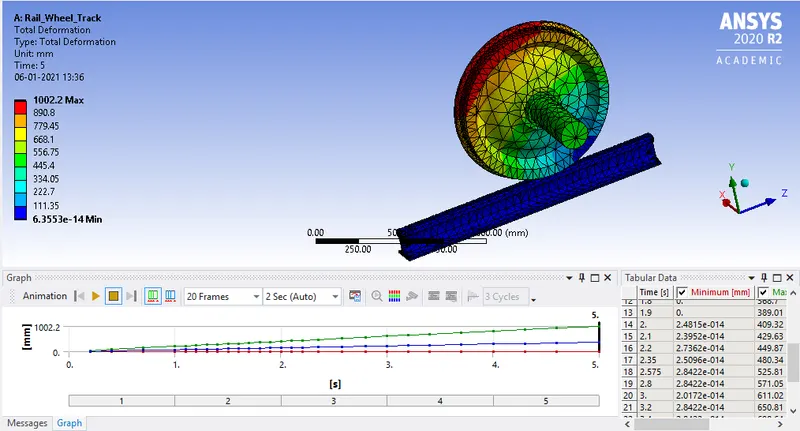
       1. Total Deformation:

       

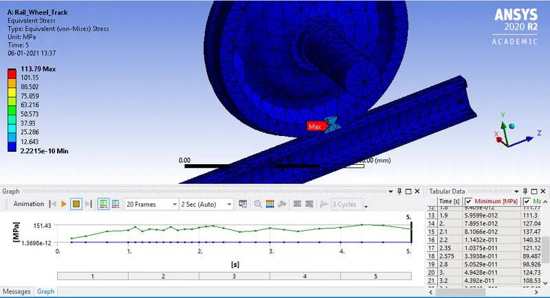
       2. Equivalent Stress:
       
       
       
       3. Equivalent Strain: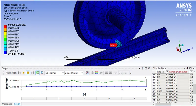
       
       
       
       4. Life of Wheel: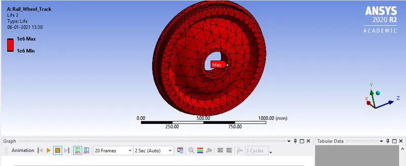
       
       
       
       

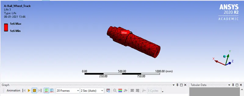
       5. Life of Shaft:

       

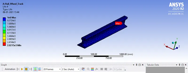
       6. Life of Track:
       
       

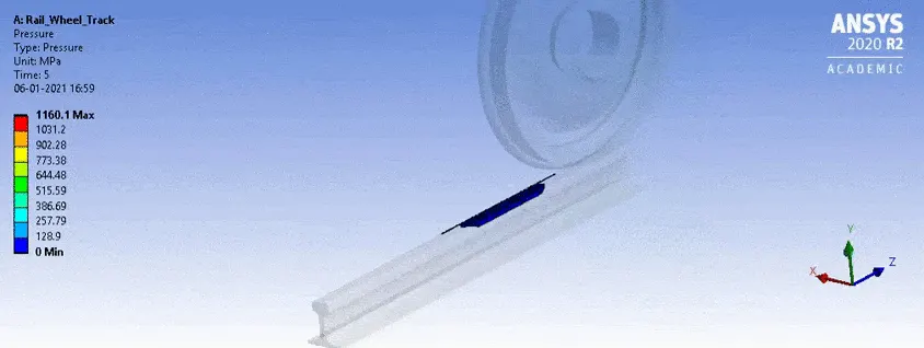
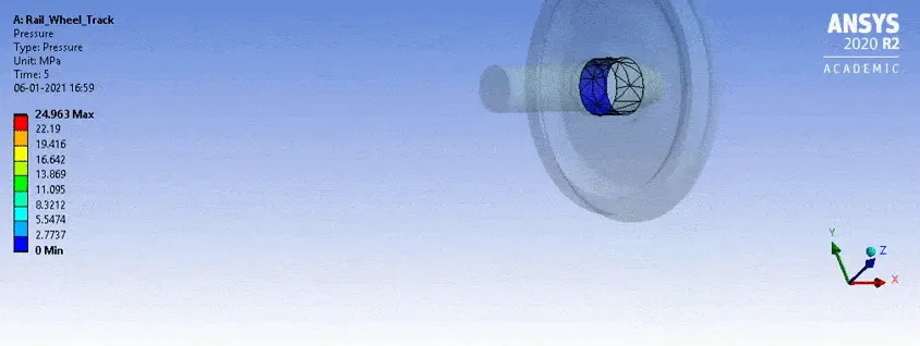
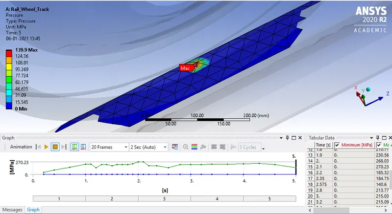
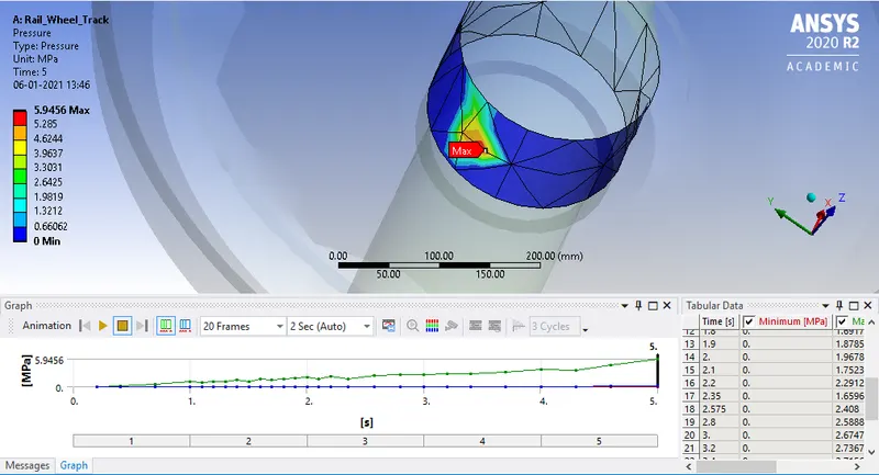
       7. Contact Pressure:
       
       

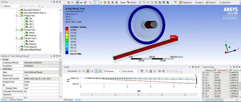
       8. User Defined Equation result (Angle):

       

    2. Case 1: b. Bearing Load of 500KN Applied.
       
       1. Total Deformation: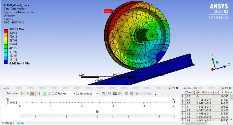
       
       
       
       2. Equivalent Stress: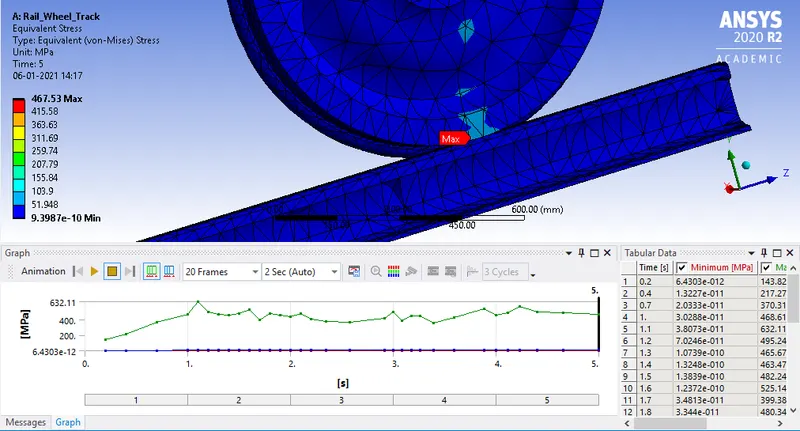
       
       
       
       3. Equivalent Strain: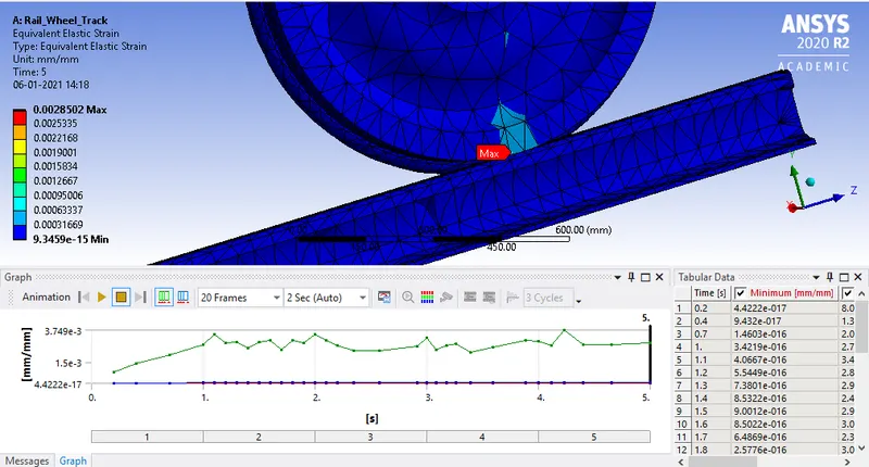
       
       
       
       4. Life of Wheel: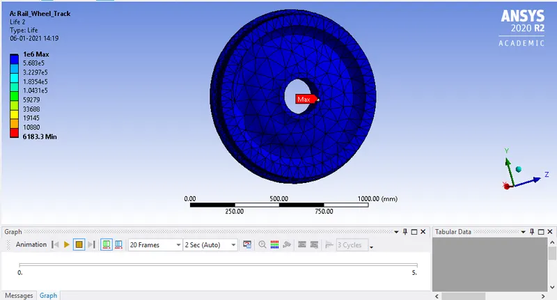
       
       
       
       5. Life of Shaft: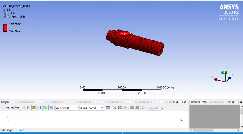
       
       
       
       6. Life of Track: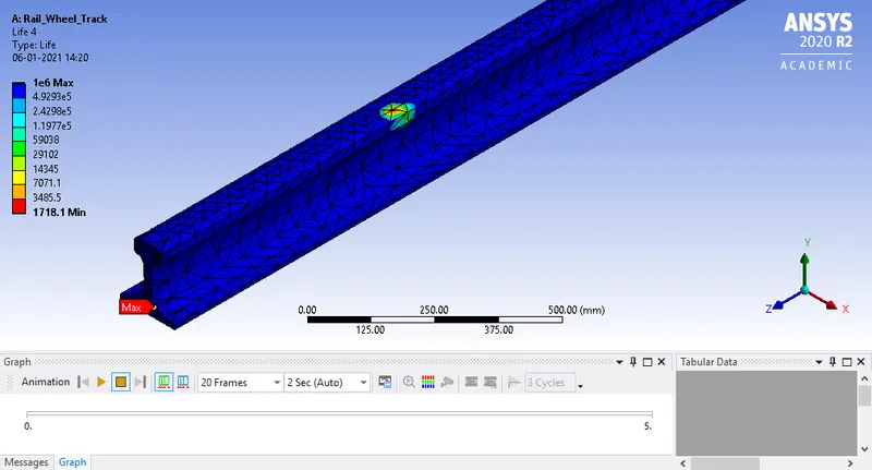
       
       
       
       7. Contact Pressure: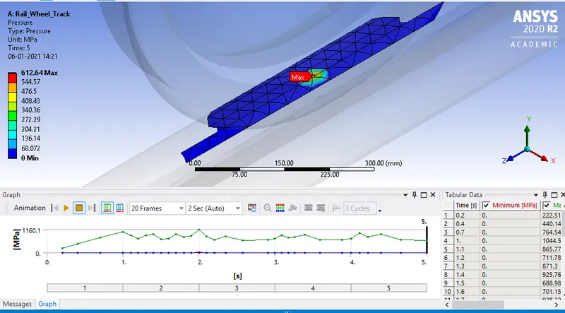
       
       
       
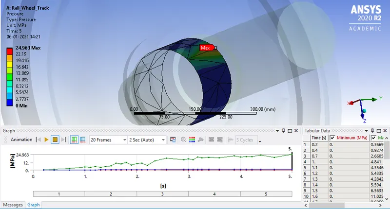
       8. User Defined Equation result (Angle):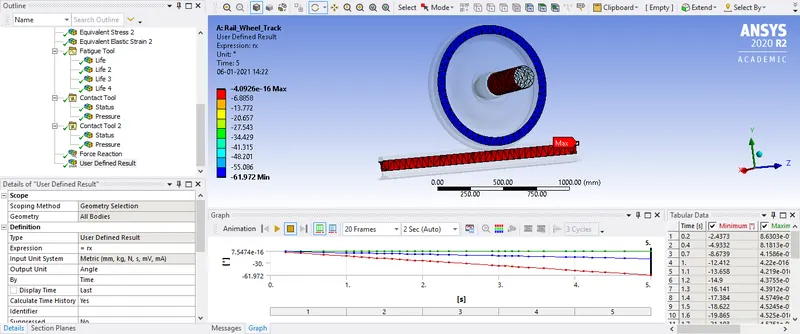
       
       
       
       

26. COMPARISON:
    
    Comparing the results for bearing load of 100KN applied and bearing load of 500KN applied:
    
    

    Bearing Load Applied	Total Deformation (mm)	Max. Equivalent Stress (MPa)	Max. Equivalent Strain	Contact Pressure at rail (MPa)	Contact Pressure at Bearing (MPa)
    100KN	1002.2	113.79	6.63e-4	139.9	5.94
    500KN	1001.9	467.53	2.85e-3	612.64	24.96

27. CONCLUSIONS from CASE - 1:
    
    1. The data as observed from the table, we can denote that the Max. Stress, Strain and Contact Pressure for the case where bearing load applied is 500KN is more than the case where the bearing load applied is 100KN.
    
    2. When comparing the life cycles, we can infer that the material assigned will be suitable for the rail wheel under both the bearing load applications as the life cycles observed are similar in both the cases.
    
    
    
    
    
    
28. Case 2: Setup for User Defined Equation Result for Total Deformation.
    
    1. Total Deformation results can be obtained using algebraic equation in the form of vector quantities.
    
    a. Let's suppose,
    Symbol for Total deformation is U.
    Deformation along X is ux.
    Deformation along Y is uy.
    Deformation along Z is uz.
    
    b. The equation for total deformation is U = `sqrt((ux)^2+(uy)^2+(uz)^2)`
    
    
    
    2. Enter the above equation in Expression Tab and change the output result to Displacement and solve for the Equation to get Total deformation.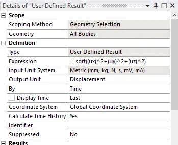
    
    
    
    
29. RESULT:
    
    1. CASE - 2: a. Bearing Load of 100KN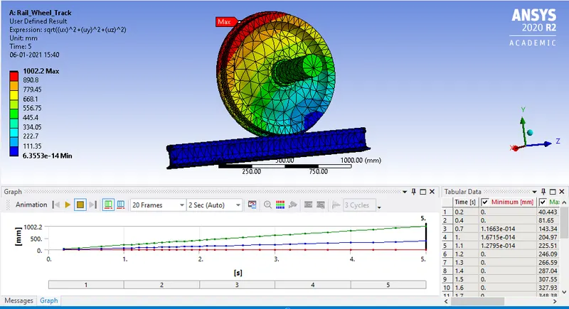
    
    
    
    2. CASE - 2: b. Bearing Load of 500KN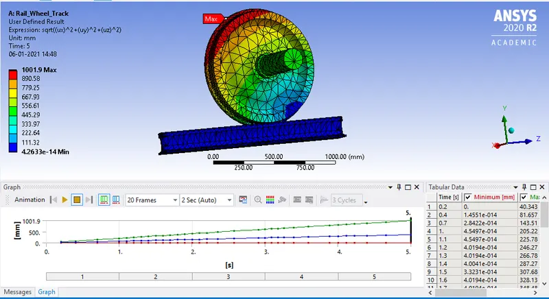
    
    
    
    
30. COMPARISON:
    
    

    Bearing Load Applied	User defined Total Deformation (mm)	Inbuilt Total Deformation (mm)
    100KN	1002.2	1002.2
    500KN	1001.9	1001.9

    
    
    
31. CONCLUSION from CASE - 2:
    
    As observed, the User defined results are same as the inbuilt results.
    
    
    
    
32. SIMULATION RESULTS:
    
    Case - 1: a. Bearing Load of 100KN:
    
    Deformation: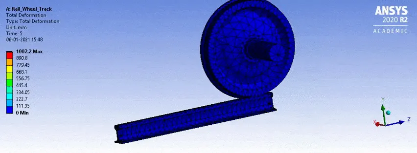
    
    
    User Defined Deformation: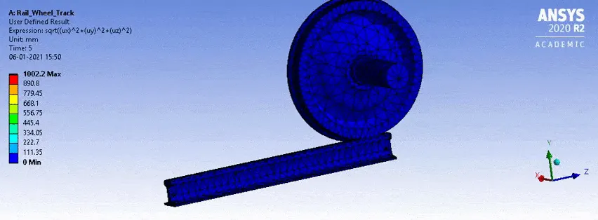
    
    
    Equivalent Stress: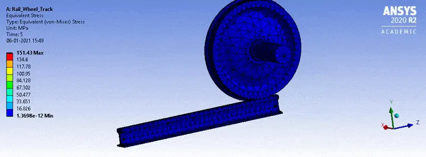
    
    Equivalent Strain: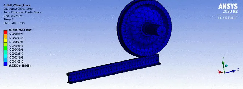
    
    Stress on Wheel: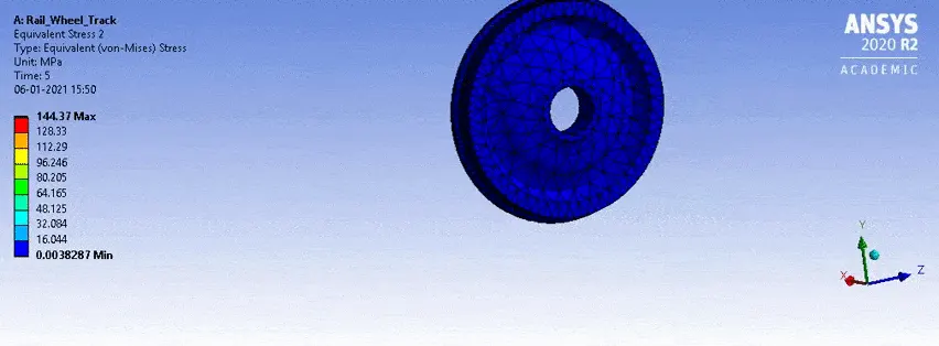
    
    Strain on Wheel: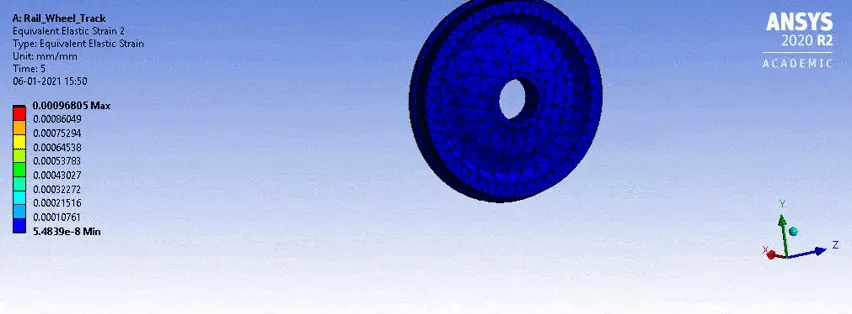
    
    Force Reaction: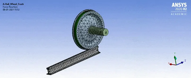
    
    
    Contact Pressure: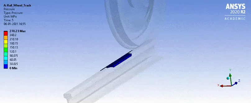
    
    
    
    
    
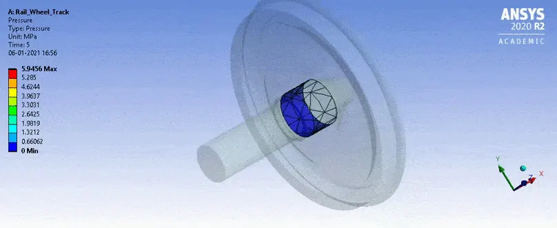
    Case - 2: b. Bearing Load of 500KN:
    
    Total Deformation: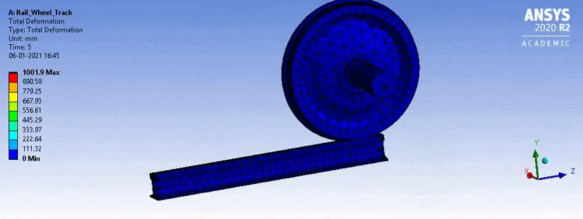
    
    User Defined Deformation: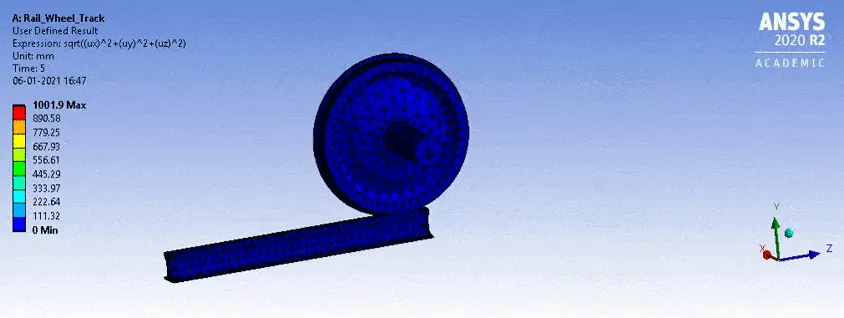
    
    Equivalent Stress: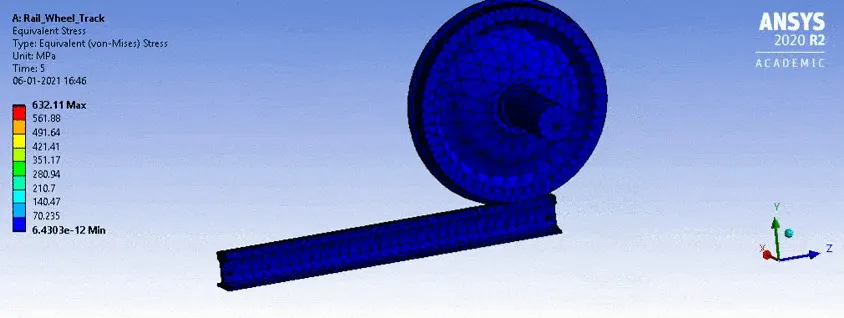
    
    Equivalent Strain: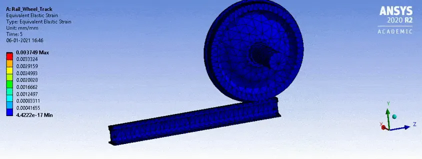
    
    Stress on Wheel: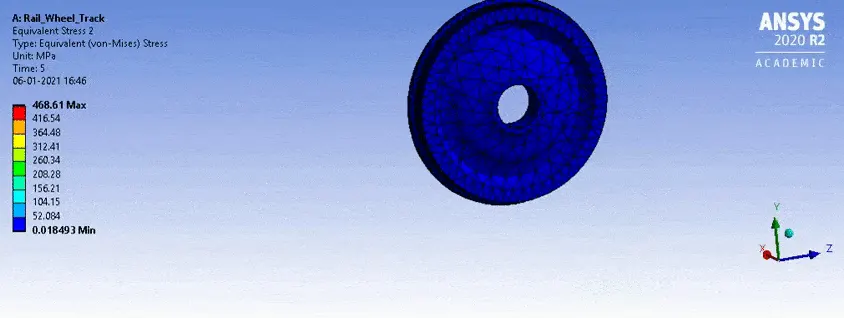
    
    Strain on Wheel: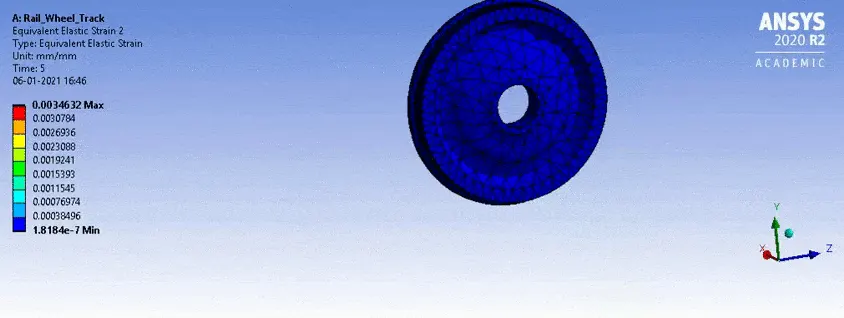
    
    Force Reaction:
    
    
    Contact Pressure: