Week 2 - OTTO CYCLE (Air standard Cycle)
AIM
To write a program that can solve an otto cycle and make plots for it.
PROCEDURE
OTTO CYCLE
An Otto cycle is an idealized thermodynamic cycle that describes the functioning of a typical spark ignition piston engine. It is the thermodynamic cycle most commonly found in automobile engines
1 - 2 Isentropic Compression
2 - 3 Constant Volume Combustion
3 - 4 Isentropic Expansion
4 - 1 Constant Volume Heat Rejection
In order to solve an otto cycle,
We start with the Engine Geometric Parameters.
- Bore
- Stroke
- Connecting Rod Length
- Compression Ratio (cr)
Once we have the above parameters, we'll be able to solve the 'kinematic equation' of the 'piston' and the 'volume trace'. And from the 'volume trace' we will be able to calculate the 'swept volume' and the 'clearance volume' from which we can calculate 'v1' and 'v2'.
Now, Let us start wrinting the program.
Under Editor> Open a new script window > First we start with the basic flow and then we assign the Input variables of gamma as '1.4'.
Now we have to define the % State variables i.e State 1. The pressure at State 1 is '1' atmosphere and the temperature is '500' kelvin. For State 1, the volume will be computed through the geometric parameters of the engine.
Next we assign the values for the bore as '0.1', stroke as '0.1', connecting rod(con_rod) as '0.15' and compression ratio(cr) as '12'.
Then we have to determine the '% Thermal efficiency' of the engine. Thermal efficiency - The efficiency of a heat engine measured by the ratio of the work done by it to the heat supplied to it.
The equation for thermal efficiency is
Thermal efficiency = 1 - (1/cr^κ-1), where κ = 1.4
And when we run the program we can see that Thermal efficiency has been calculated.
Now we have to calculate the swept volume(v_swept) and the clearance volume(v_clearance). Swept volume is the volume of the cylinder which is defined by the bore and stroke.
v_swept = (pi/4)*bore^2*stroke
'Clearance volume' is calculated with 'Swept volume' divided by 'cr - 1'
Total volume is nothing but the 'swept volume' + 'clearance volume' which is equal to 'v1'. And 'v2' is the volume of top dead center which is the 'clearance volume'. Now the state variable of state 1 has been calculated.
Then we have to calculate the % State variable for state 2. The pressure in state 2 can be computed using the relation p1v1 power gamma which is equal to p2v2 power gamma that defines the isentropic compression process. From this we can determine that p2 is equal to p1 multiplied with v1 by v2 whole power gamma. where p2 is equal to p1 multiplied by compression ratio power gamma. v1 and v2 is the compression ratio. Now when we run the program we can see that p2 is greater than p1.
Then to compute the temperature in state point 2, we will be using the Ideal Gass Law. Since p1 by t is constant, we determine that p1v1 by t is equal to p2v2 by t2.
%p1v1/t1 = p2v2/t2 | t2 = p2*v2*t1/(p1*v1)
Take t2 = p2*v2*t1/(p1*v1) and run the program. We can see that t2 is computed in the command window.
Now we have to determine the % State variable at state point 3. The state point 3 represents the end point of the constant volume combustion process. So, v3 is equal to v2.
Inorder to process our calculation, we should assume that the end of the combustion process the temperature change is 2000 kelvin and hence t3 is set as 2300 kelvin in our input.
Next the only % State variable that we have to determine at state point 3 is pressure which can be determined by the Ideal Gass Law.
%p3v3/t3 = p2v2/t2 | p3 = p2*t3/t2
Take
p3 = p2*t3/t2 and run the program. We can see that p3 is computed. Here the value of p3 is higher than p2. Since the combustion process takes place, the pressure is going to be highest.
Finally we have to compute the % State variables at the state point 4. The volume at state 4 is equal to state 1. v4 is equal to v1.
To compute the pressure at state 4 we determine that
%p3v3^gamma = p4v4^gamma | p4 = p3*(v3/v4)^gamma
Take
p4 = p3*(v3/v4)^gamma and run the program. p4 is determined. so now we have all four state variables to make a plot for the air standard cycle.
Open a new figure window 'figure(1)' and add the 'hold on' command. Write plot(v1,p1,'.','color','r') Here we input plot variables for volume, pressure, '.' plot pint symbol and the color of the plot as red. So we have plot four state variables. Also set xlabel as 'V' and ylabel as 'P'. when we run the program we can see that the plots are visible as shown in the below Fig.
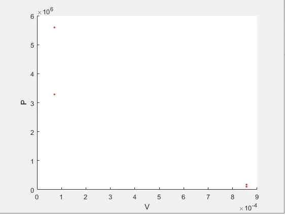
As of now we have managed to plot the individual state points. Now we have to write a program to join the plot points. Here we are going to use piston kinematics equation to determine the curve from top dead center to the bottom dead center. This process shows how the combustion chanmber volume changes as a function of a crank angle.
CALL FUNCTION program for ENGINE KINEMATICS
Under Editor> Open a new script window > Here we write
function [V] = engine_kinematics(bore, stroke, con_rod, cr, start_crank, end_crank)
[V] - volume trace (output)
engine_kinematics - function name
(bore, stroke, con_rod, cr, start_crank, end_crank) - Inputs
write a = stroke/2 - where 'a' crank in radius is the stroke divided by two.
R = con_rod/a - where 'R' is the ratio of connecting rod length to the crank in radius 'a'
Then calculate the swept volume and clearance volume as we did before.
v_s = pi/4*bore^2*stroke;
v_c = v_s/(cr-1)
Now run the program. we can see that v_c and v_s has been calculated.
let us assume that theta = linspace(start_crank,end_crank,100)
Here we use a particular formulae that determines how the volume inside an engine combustion chamber is going ot change.
This formulae is derived from geomentric relations.
V/Vc = 1 + 1/2(rc-1)[R+1-cosd(theta) - (R^2 - sind^2(theta))^0.5]
Here we are going to split the formulae into three terms i.e term1 = 0.5*(cr-1), term2 = R + 1 - cosd(theta), term3 = (R^2 - sind(theta).^2).^0.5
Our volume trace is going to be equal to (1+ term1*(term2 - term3)).*v_c i.e the entire term is multiplied by the clearance volume 'v_c'. End the function with end command.
whenever we want to substitute different values we call the function which is a template. Calling the function is using the function with appropriate values.
Now we call the function in otto cycle program
where In state point 2 we determine constant_c = p1*v1^gamma
V_compression = engine_kinematics(bore, stroke, con_rod, cr,0,180)
P_compression = constant_c./V_compression.^gamma
since P_compression is an array we use '.' element while operator.
Now let us go to the first plot and write
plot(V_compression, P_compression) and run the program we get the compression curve.
Like wise we do the same for the expansion process in state point 3
constant_c = p3*v3^gamma
V_expansion = engine_kinematics(bore, stroke, con_rod, cr,180,0)
P_expansion = constant_c./V_expansion.^gamma
In plot 3 write
plot(V_expansion, P_expansion) and run the program we get the expansion curve. like so we have to plot the curve for constant volume combustion as plot([v2,v2],[p2,p3],'color','r') and constant volume heat rejection as plot([v4,v4],[p4,p1],'color','r') now run the program to get the complete otto cycle.
SCRIPT WINDOW - OTTO CYCLE
clear all
close all
clc

% Inputs
gamma = 1.4
t3 = 2300

% State variables
p1 = 101325
t1 = 500

% Engine geometric parameters
bore = 0.1;
stroke = 0.1;
con_rod = 0.15;
cr = 12;

% Thermal efficiency
thermal_efficiency = 1 - (1/cr^0.4)

% Calculating the swept volume and the clearance volume
v_swept = (pi/4)*bore^2*stroke;
v_clearance = v_swept/(cr-1);

v1 = v_swept +  v_clearance
v2 = v_clearance

% State variables at state point 2
% p2v2^gamma = p1v1^gamma
% p2 = p1*(v1/v2)^gamma = p1*cr^gamma
p2 = p1*cr^gamma;

%p1v1/t1 = p2v2/t2 | t2 = p2*v2*t1/(p1*v1)
t2 = p2*v2*t1/(p1*v1)

constant_c = p1*v1^gamma;
V_compression = engine_kinematics(bore, stroke, con_rod, cr,0,180);

P_compression = constant_c./V_compression.^gamma;


% State variables at state point 3
v3 = v2

%p3v3/t3 = p2v2/t2 | p3 = p2*t3/t2
p3 = p2*t3/t2

constant_c = p3*v3^gamma;
V_expansion = engine_kinematics(bore, stroke, con_rod, cr,180,0);

P_expansion = constant_c./V_expansion.^gamma;

% State variables at state point 4
v4 = v1

%p3v3^gamma = p4v4^gamma | p4 = p3*(v3/v4)^gamma
p4 = p3*(v3/v4)^gamma

figure(1)
hold on
plot(v1,p1,'.','color','r')
plot(V_compression, P_compression)
plot(v2,p2,'.','color','r')
plot(v3,p3,'.','color','r')
plot(V_expansion, P_expansion)
plot(v4,p4,'.','color','r')
plot([v2,v2],[p2,p3],'color','r')
plot([v4,v4],[p4,p1],'color','r')
xlabel('V')
ylabel('P')
SCRIPT WINDOW - CALL FUNCTION FOR ENGINE KINEMATICS
function [V] = engine_kinematics(bore, stroke, con_rod, cr, start_crank, end_crank)


a = stroke/2;
R = con_rod/a;

v_s = pi/4*bore^2*stroke;
v_c = v_s/(cr-1)


theta = linspace(start_crank,end_crank,100);

term1 = 0.5*(cr-1);
term2 = R + 1 - cosd(theta);
term3 = (R^2 - sind(theta).^2).^0.5;


V = (1+ term1*(term2 - term3)).*v_c;


end
COMMAND WINDOW - OTTO CYCLE
gamma =

    1.4000


t3 =

        2300


p1 =

      101325


t1 =

   500


thermal_efficiency =

    0.6299


v1 =

   8.5680e-04


v2 =

   7.1400e-05


t2 =

   1.3510e+03


v_c =

   7.1400e-05


v3 =

   7.1400e-05


p3 =

     5593140


v_c =

   7.1400e-05


v4 =

   8.5680e-04


p4 =

   1.7251e+05

>>
WORKSPACE - OTTO CYCLE
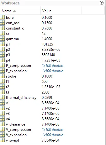
PLOT GRAPH - INDIVIDUAL STATE POINTS
PLOT GRAPH - OTTO CYCLE
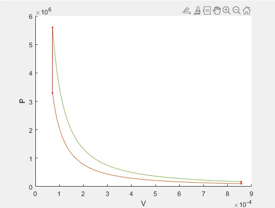
1 - 2 Isentropic Compression
2 - 3 Constant Volume Combustion
3 - 4 Isentropic Expansion
4 - 1 Constant Volume Heat Rejection
Otto cycle solved by code using MATLAB. Thermal efficiency of the engine is 0.6299
No errors found.