Flow over a Cylinder

Aim

• Simulate the flow over the cylinder and explain the phenomenon of Karman vortex street.
• Firstly, Simulate the flow with the steady and unsteady case and calculate the Strouhal Number for Re=100
• Secondly, calculate the coefficient of drag and lift over a cylinder by setting the Reynolds number to 10,100,1000,10000 and 100000 (Run with steady solver)
• Next, discuss the effect of Reynolds number on the coefficient of drag. [Result should be validated with any standard literature and error should be within 5%]
• In both approaches, show that the flow has converged. Mention the quantities or plot which determine that the flow has converged.
• Plot the coefficient of drag and lift.
• Plot to show vortex shedding behind the cylinder.

Objective

• Study and understand the simulation of flow over the cylinder and the phenomenon of Karman vortex street.
• Create a 2D geometry in the design modeler as per the given dimensions.
• Generate proper mesh with an effective inflation layer over the cylinder wall.
• Simulate solution into two-part: in the first part, simulate the flow with steady and transient case and calculate the Strouhal Number for Re=100
• In the second part, calculate the coefficient of drag and lift over a cylinder by setting all given Reynolds numbers using a steady solver.
• Discuss the effect of Reynolds number on the coefficient of drag.
• Also, show the flow has converged with the help of the quantities or plot which determine that the flow has converged.
• Plot the graph for the coefficient of drag and coefficient of lift.
• Plot to show vortex shedding behind the cylinder.
• Lastly, write a detailed report which explains all the findings of the project.

This report emphasis on the analysis of two-dimensional flow over a circular cylinder in different Reynolds number. The analytical solution of the same case modeled with the potential flow is known and easy to interpret; however, the physical mechanism which rules real flow around a circular cylinder, as well as its mathematical treatment, is highly complex. Some examples are the boundary layer detachment and oscillatory effects that without a CFD study would be very difficult to determine either analytically or experimentally.

The unconfined or free flow past a circular cylinder exhibits a rich variety of flow regimes depending upon the intrinsic nature of the flow. It needs to be emphasized here that at finite Reynolds number, two flow regimes can be identified in the vicinity of the cylinder, i.e., the boundary layer of thickness, which is usually much smaller than the diameter of the cylinder and the wake region which is of the order of one-to-two times the diameter. Notwithstanding the fundamental significance of delineating the conditions for the transition from one flow regime to another, this information is also germane to develop the scaling laws for the gross engineering parameters like drag and lift coefficients, Strouhal number, and Nusselt number with the Reynolds number and Prandtl number. Therefore, significant research effort has been expended on exploring this aspect in this field. It is thus instructive to recapitulate the key points pertaining to the onset and distinguishing features of various flow regimes documented for the uniform transverse flow of Newtonian fluids past an unconfined smooth circular cylinder which is long in the transverse direction thereby eliminating the complications arising from the surface roughness and end effects, respectively.

For the aforementioned simple flow, the flow is governed by the familiar Reynolds number.

`Re_L = (UL)/v_o`

Where,

U = the free stream flow speed.

L = a characteristic length parameter of the body or channel

`v_o` = the free stream kinematic viscosity parameter of the fluid

`v_o = (mu_o)/(rho_0)`

`rho` = fluid density

`mu_o` = dynamic viscosity

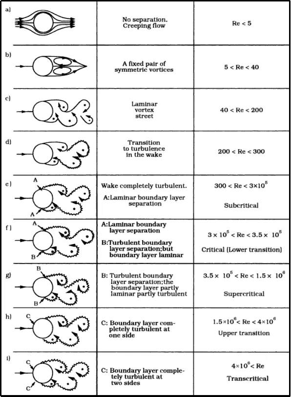
As the value of the Reynolds number is progressively incremented, the viscous effects gradually weaken, and fluid inertia increases, and naturally, a fluid element is no longer able to negotiate the sudden changes in body shape without incurring losses in its momentum (or kinetic energy). Therefore, a point is reached when due to the diverging area, an adverse pressure gradient is established in the rear of the cylinder thereby leading to the detachment of flow to the surface of the cylinder. The location of the point of separation coincides with that of the change of the sign of the velocity on the surface of the cylinder

The following figure shows the schematics of the different flow regimes past an unconfined circular cylinder.

Karman vortex street

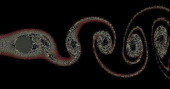
In fluid dynamics, a Karman vortex street is a repeating pattern of swirling vortices, caused by a process known as vortex shedding, which is responsible for the unsteady separation of flow of a fluid around blunt bodies.

A vortex street will form only at a certain range of flow velocities, specified by a range of Reynolds numbers (Re), typically above a limiting Re value of about 90. The (global) Reynolds number for a flow is a measure of the ratio of inertial to viscous forces in the flow of a fluid around a body or in a channel and may be defined as a nondimensional parameter of the global speed of the whole fluid flow.

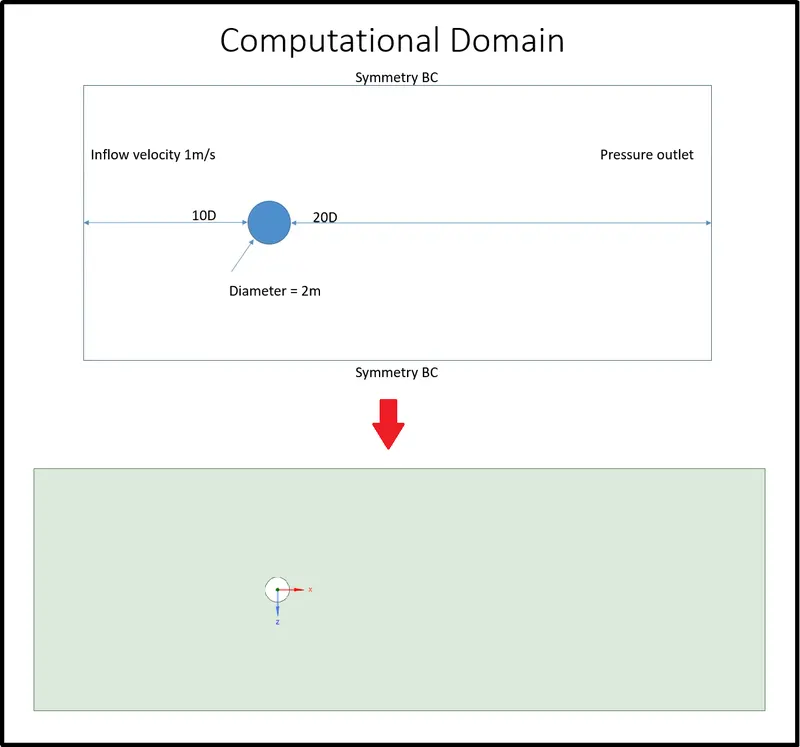
Geometry Creation:-

From this point, we can start our project by creating our geometry in space claim using given dimensions.

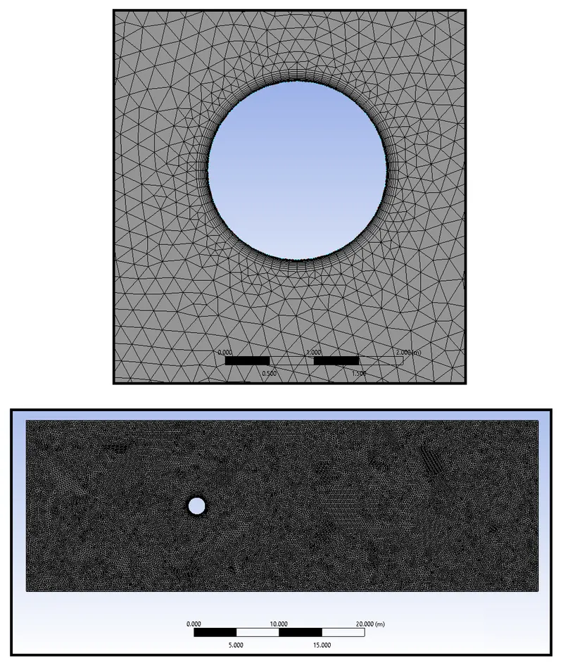
Meshing:-

In meshing mesh the 2D model b providing the proper size and type of the mesh. Also, provide inflation layers on the cylindrical wall to capture the wall boundary nicely.

Problem Setup:-

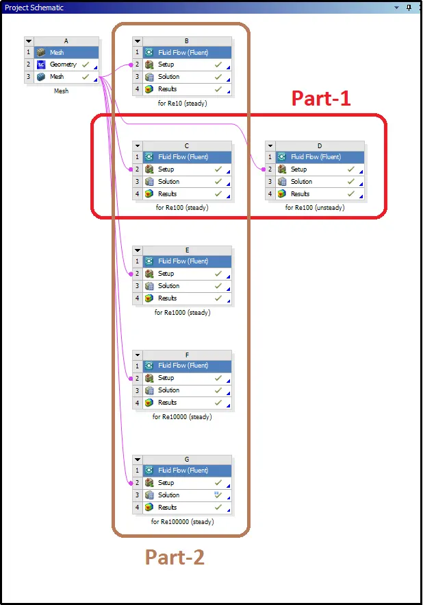
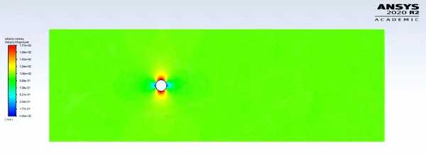
PART-1-Case 1

Simulation of flow for the steady condition for Re=100.

for all simulations, let us consider a working fluid as air. Air has a density of approximately 1 kg/m^3 and considers the viscosity of air as 0.02mPa.

`Re_L = (UL)/v_o`

`U = (Re_L xx ((mu_o)/(rho_0)))/L`

In this case, our diameter of the cylinder is 2m so our characteristic length will be 2m

`U = (100 xx (0.02/1))/2`

`U = 1`m/s

PART-1-Case 2

Simulation of flow for the unsteady or transient condition for Re=100.

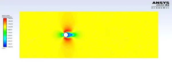
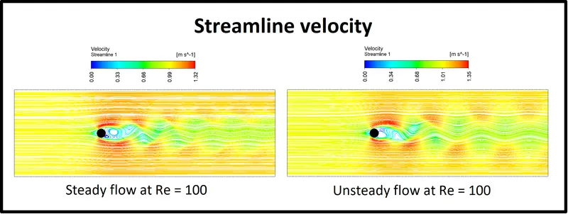
After simulation for both cases, let us compare the results.

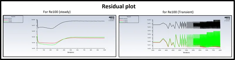
As we can see in the residual plot, there are too many differences in both steady and transient states. In a steady-state solver, we can say that the solution is converged after 550 iterations. On the other hand, in the case of a transient solver, it is very hard to understand that if the solution is converged or not. That why in the simulation we need t monitor points behind the cylinder to calculate the measuring parameters are getting repeated results (results with the same frequency) or not. Observing results at monitor points can help us to gain the confidence of converged results. Let us see from which iteration our results are getting converged by observing the following graph of velocity at the monitor point behind the cylinder at the distance of 8m from the cylinder center.

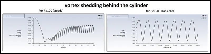
In the first graph, the frequency of velocity is repeating itself along straight right direction after 700 iterations in that case we can say that the solution is converged for the steady case. And for, transient simulation the velocity frequency is constant, which will be going to increase with respect to time so we can run the simulation for the required number of times to analyze the flow varies according to time.

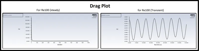
If we compare both steady and transient cases with respect to its drag coefficient, at a steady-state drag is almost constant after 80 iterations. On the other side, in transient solution, it is varying in a small frequency with respect to the time. But both solutions almost showing the same value for the drag.

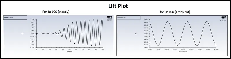
In lift plot, steady solution improving frequency gradually from zero to +-0.25 (approx), and after the 800^th iteration, it is showing stable results. For transient simulation, the resulting frequency is the same from the starting and going forward with the same sin wave. Also, the magnitude of the curve of the transient solution is high, about+-0.4, than the curve of the steady solution.

The strouhal number

The strouhal number represents the ratio of inertial force due to the local acceleration of the flow to the inertial forces because of the convective acceleration.

Depending on the time scale of the problem, this ratio may be order unity, and therefore its importance is not obvious.

Inflows characterized by a periodic motion, the Strouhal number is associated with the oscillation of the flow due to the inertial forces relative to the changes in velocity due to the convective acceleration of the flow field. Thus, an alternative definition of the Strouhal number better suited to periodic flows is given by the following expression

`S_(tr) = (fL)/U`

Where,

f is the frequency of the oscillation with dimensions [T^-1].

And, such oscillations are found in vortex street wakes behind bluff bodies which we are studying in this project.

At high Strouhal numbers oscillation dominate the flow while at low Strouhal number the oscillation is swept by the fast-moving fluid.

In Fluent, one can directly calculate Strouhal Number using Lift calculated data and plot the results.

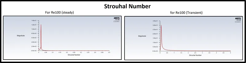
Steady-state simulations are typically performed to get the conclusive, intermediate solution which is not time accurate. this means if any particular iteration solution shows any specific value of velocity then that value of velocity does not co-relate to a particular time. And this is all because of which simulation is not giving accurate results. but in the transient case, the solution gets solved with time and changes with time. This gives accurate results than steady simulation. in such a flow regime, to resolve the vortex shedding characteristics the time-dependent momentum equations are always preferable.

PART-2-Case 1

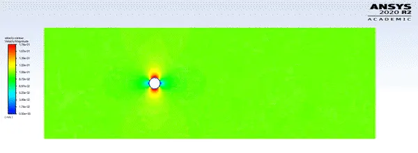
Simulation of flow for the steady condition for Re=10.

Calculate velocity for Reynolds number = 10

`Re_L = (UL)/v_o`

`U = (Re_L xx ((mu_o)/(rho_0)))/L`

`U = (10 xx (0.02/1))/2`

`U = 0.1`m/s

PART-2-Case 2

Simulation of flow for the steady condition for Re=100.

Calculate velocity for Reynolds number = 100

`Re_L = (UL)/v_o`

`U = (Re_L xx ((mu_o)/(rho_0)))/L`

`U = (100 xx (0.02/1))/2`

`U = 1`m/s

PART-2-Case 3

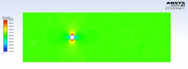
Simulation of flow for the steady condition for Re=1000.

Calculate velocity for Reynolds number = 1000

`Re_L = (UL)/v_o`

`U = (Re_L xx ((mu_o)/(rho_0)))/L`

`U = (1000 xx (0.02/1))/2`

`U = 10`m/s

PART-2-Case 4

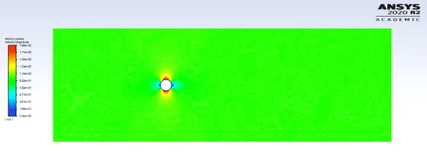
Simulation of flow for the steady condition for Re=10000.

Calculate velocity for Reynolds number = 10000

`Re_L = (UL)/v_o`

`U = (Re_L xx ((mu_o)/(rho_0)))/L`

`U = (10000 xx (0.02/1))/2`

`U = 100`m/s

PART-2-Case 5

Simulation of flow for the steady condition for Re=100000.

Calculate velocity for Reynolds number = 100000

`Re_L = (UL)/v_o`

`U = (Re_L xx ((mu_o)/(rho_0)))/L`

`U = (100000 xx (0.02/1))/2`

`U = 1000`m/s

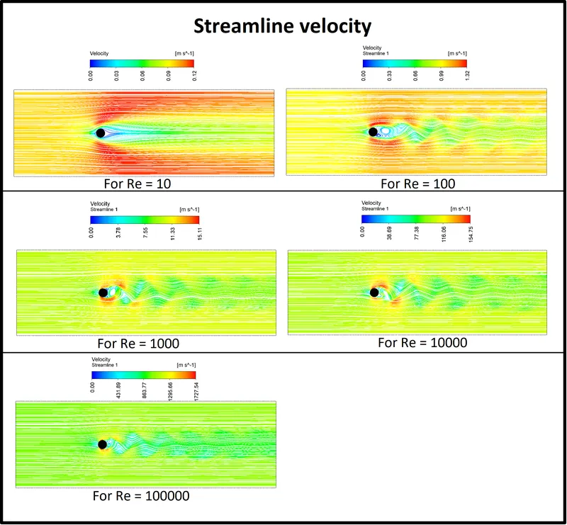
At Re = 10, the flow is still a bit laminar but a visible separated (wake) flow region appears in the rear of the cylinder. Therefore the flow no longer exhibits the fore and aft symmetry, albeit it is still symmetric about the mid-plane. As the value of the Reynolds number is increased further, the wake region is characterized by a pair of counter-rotating vortices that remain attached

At Re = 100, the wake becomes unstable (initially originating from the downstream end) and the viscous forces are no longer sufficient to quash these disturbances. The instability grows further with the increasing Reynolds number. the flow is still laminar and two-dimensional. However, one needs

to solve the time-dependent momentum equations to resolve the vortex-shedding characteristics in this flow regime.

Further increase in the value of the Reynolds number induces increased levels of turbulence in the boundary layer and wake region.

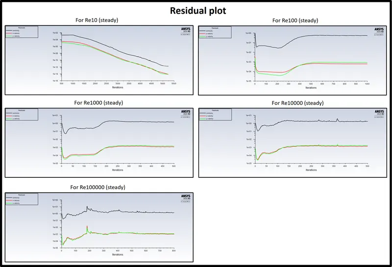
As we discussed above, in a vortex street simulation we most probably never get our results fully converged. therefore, we need to use the alternate option to see our results are converged or not. as we can notice in the above plots of residuals, at first plot residuals are not constant at all. but if we notice the velocity results at the monitor point behind the cylinder, there is a constant velocity after 1500 iterations.

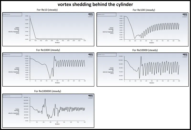
In the above vortex shedding chart, all the results at constant frequency repeating themselves. therefore, we can consider at this point our results are converged.

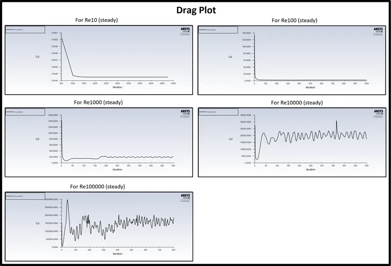
Drag Coefficient

The drag coefficient is a dimensionless factor of proportionality between the overall hydrodynamic force vector on a body in a liquid or gas flow and the product of the reference area of the body and velocity head.

Effect of Reynolds number on the drag coefficient.

The above plots exhibit, drag plots for Reynolds number 10,100,1000,10000, and 100000. If the Reynolds Number is large, the viscosity effect is small. In practical values the inertia or density forces dominate, and the parasite drag increases with the square of the velocity. However, although the viscosity is unimportant, it may still affect the very thin boundary layer, leading to the creation of turbulent flow. Thus the importance of the Reynolds Number is that it tells us the type of flow we can expect. It tells you whether you can hope for having laminar flow over the wing and other parts of your airplane. A low Reynolds Number gives laminar flow while a high Reynolds Number gives turbulent flow. For both a laminar and a turbulent boundary layer increasing Reynolds Number gives lower skin friction drag. However, because of the higher energy loss in the boundary layer, a turbulent layer always has higher skin friction drag.

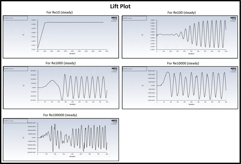
As depicted in the above plots, the lift is also an oscillating entity, and its oscillation with the same frequency after a particular iteration for each plot. one can observe that the frequency and the oscillation increase with rising in Reynold's number.

it can also be observed that the average lift value was nearly zero for the low Re number but it raises to a positive value with an increase in Reynold's number.

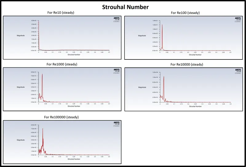
By using Lift data, we can directly calculate the values for the Strouhal Number using FFT plot results in Ansys. The Strouhal number of a stationary tube or circular cylinder is a function of Reynolds number but less of surface roughness and freestream turbulence.

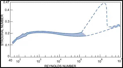
The variation in the Strouhal number is associated with the changes in the flow structure. From Figure 2 it is found that the Strouhal number is about 0.2 over a large Reynolds number interval. In the Reynolds number range 250 < Re_D < 2×10⁵ the empirical formula.

`S_r = 0.198(1-(1.9)/(R_(eD)))`

is sometimes recommended for the estimation of the Strouhal number. At high Reynolds numbers, the vortex shedding does not occur at a single distinct frequency but rather over a narrow band of frequencies.

Conclusion:-

• Basic understanding of space claim about modeling simple CAD geometry.
• Study of good implementation of meshing on the geometry according to the region of simulation results.
• Karman Street Phenomenon for flow over cylinder studied and observed in this project.
• In a comparison of steady-state and transient methods, analyzing a laminar flow, for Reynolds number more than 100 it is vital to use the time-dependent momentum equations to resolve the vortex-shedding characteristics
• As the Reynolds number increased further, the vortices are shed alternately from the upper and lower cylinder surface at a definite frequency depending on the Reynolds number. And for the value of Re more than 1000, the flow starts to transform from laminar to turbulent.
• Furthermore, as the Reynolds number increases the inertial forces start to dominate over viscous forces which leads to a significant increase in drag and also, a rise in fluctuation in the coefficient of lift.
• Lastly, with the streamlined plot, we can observe that with the increase in the value of the Reynolds number the flow becomes more unsymmetrical which induces increased levels of turbulence in the boundary layer and wake region.

References:-

[1] Numerical simulation of laminar flow past a circular cylinder - https://www.sciencedirect.com/science/article/pii/S0307904X08000243

[2] Flow regimes - https://www.sciencedirect.com/science/article/pii/B9780123815293000049

[3] Strouhal number - https://www.sciencedirect.com/topics/engineering/strouhal-number#:~:text=Strouhal%20number%20is%20defined%20as,is%20the%20free%2Dstream%20velocity