Week 2 - Flow over a Cylinder.
AIM:
Simulate the flow over a cylinder and explain the phenomenon of Karman Vortex Street.
PART-I
Simulate the flow with the steady and unsteady case and calculate the Strouhal Number for Re= 100.
PART-II
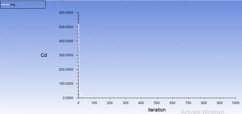
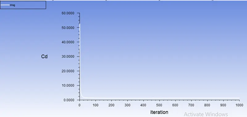
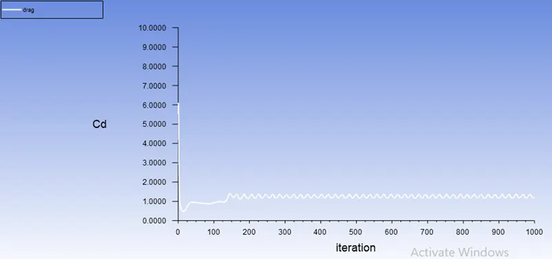
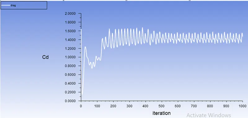
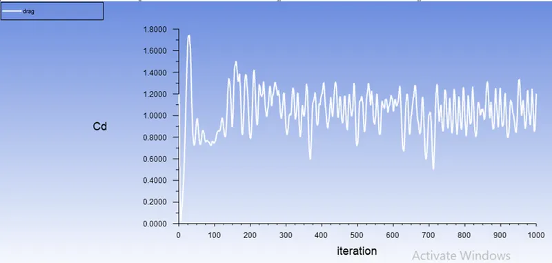
Calculate the coefficient of drag and lift over a cylinder by setting the Reynolds number to 10,100,1000,10000 & 100000. (Run with steady solver)
Discuss the effect of Reynolds number on the coefficient of drag. [Results should be validated with any standard literature and error should be within 5 %]
Expected results:-
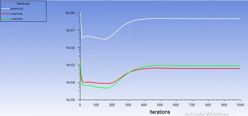
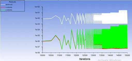
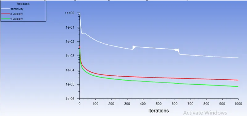
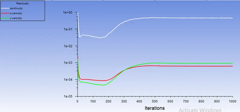
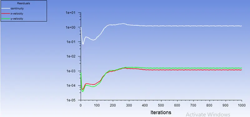
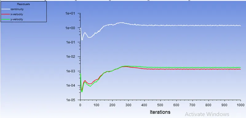
In both approaches, show that the flow has converged. That is, what quantities or plots need to be looked at to determine that the flow has converged?
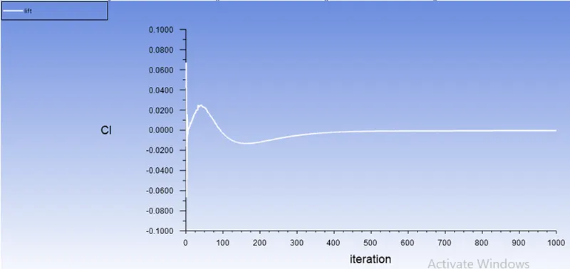
Plots of the coefficient of drag and lift.
Plots to show vortex shedding behind the cylinder.
Mention the referred material (Reference Paper or Fluid Mechanics Textbook) at the end of the challenge submission page.
Introduction:
The presence of friction in the flow causes a shear stress at the surface of the body this is known as skin friction drag. This friction is also causes another phenomenon is called Flow separation. The real flow field about a sphere is dominated by the separated flow on the rearward surface.
Flow over a cylinder is important in many industrial applications like cooling of iron or cylindrical pipe. High temperature flue gases flow over a circular cylinder in a cross flow. Depending on flow rate, fluid properties and cylinder size, the flow can be laminar, transition and turbulent.
Vortex Shedding:
When air flows around an object, there is a range of flow velocities for which a von Karman vortex street is formed.
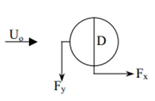
Consider a steady flow Uo on a bluff body with diameter D
Von Karman Street: Unsteady non-symmetric wake of staggered array of vortices.
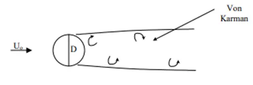
The fluid flow past the object creates alternating low-pressure vortices on the downstream side of the object. It is named after the engineer and fluid dynamitist Theodore von Karman. A vortex street is a phenomenon that forms when a turbulent flow of fluid around a body or in a channel. A vortex street will form only at a certain range of flow velocities, specified by a range of Reynolds numbers.
Reynolds number:
The Reynolds number for a flow is a measure of the ratio of inertial to viscous forces in the flow of a fluid. Larger vortexes are found at lower Reynolds number.
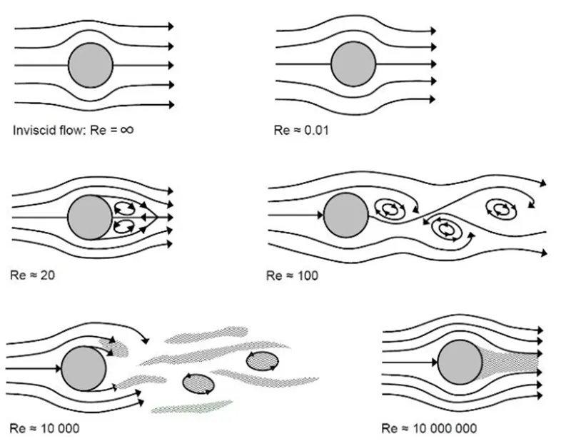
Pre processing Approach:
Model approach:
In an Ansys Fluent workbench open the geometry for model preparation.
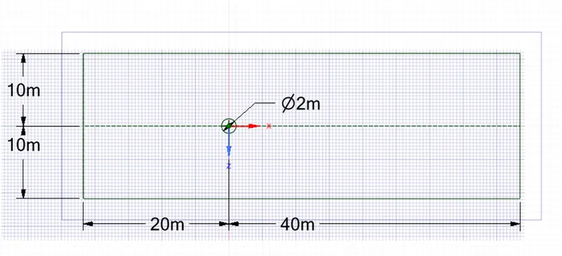
As per requirement geometry is prepared in the space claim using circle and rectangle option. This geometry is updated to generate the mesh.
MESH:
The model is primarily meshed by using the default mesh because to see how the mesh has been generate to the body based on that the mesh is improved.
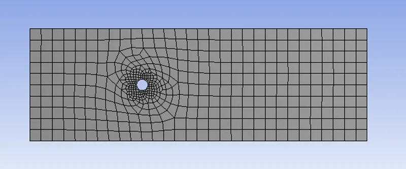
The default mesh generated is quadrilateral and around the cylinder that is somewhat polygonal shape has been generated. Hence therefore the mesh should be modified. This can been done by the above steps.
- Adding the mesh method
- By inserting the sizing
- By adding inflation
Mesh method:
Here the mesh method is changed from quadrilateral element to triangular element. Tri mesh type is preferred in the case where geometry function is quite easy and less complex, mostly for regular geometrical shapes. Contrary to that quad mesh give us relatively accurate results, and are more used in complex systems.
Sizing:
Sizing options provide greater control over the properties of a mesh as well as its size and shape. Mesh growth (transition between small and large sizes based on a specified growth rate). Curvature based refinement and angles between normals for adjacent mesh elements (curvature-based sizing).
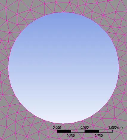
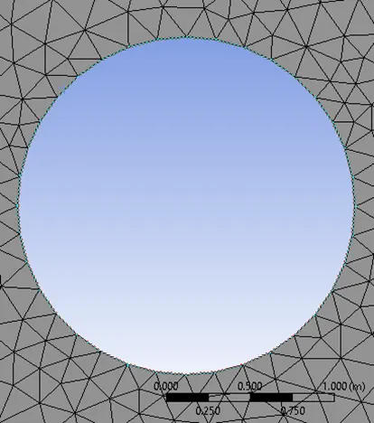
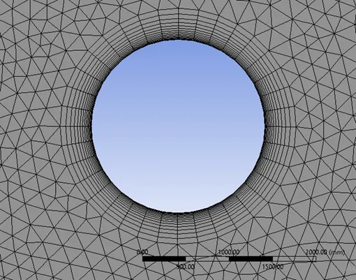
Here sizing is provided for the cylinder because to make the cylinder shape should be refined from polygon shape to circular shape by increasing the no of divisions from 1 to 36. This is calculated by dividing a circle of 3600 into equals parts of 100.
 |
 |
Inflation:
The Inflation function in ANSYS Fluent allows you to stack elements and cells in a unique way. An inflating layer can be created by trapping the normal gradient close to no-slip barriers. Only thin elements and a small number of elements can be used to achieve this.
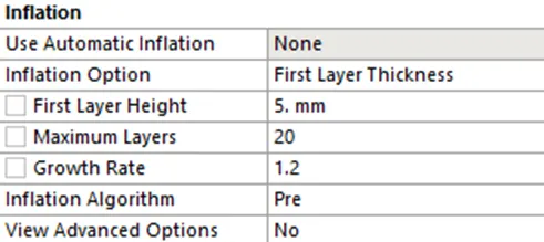
In this model inflation is provided to the circle where the mesh around the circular cylinder should be generated by layer by layer so that the flow around the cylinder is observed. The first layer of thickness is provided as 5mm, and maximum layers is around 20 and the growth rate is 1.2.where growth rate is increasing the mesh 20% more than the previous one. The mesh is generated and updated for the solution.
 |
 |
Set up:
By setting some boundary conditions the problem can be solved.
Boundary conditions:
|
Solver |
Steady state, Pressure Based |
|
Mesh |
Tria Element type |
|
Turbulence(viscosity) |
laminar |
|
Material |
Fluid(Air) |
|
Outlet velocity |
Atmospheric Pressure(atm) |
|
Diameter of cylinder |
2mt |
|
Density |
1kg/m3 |
|
Viscosity |
0.03kg/m-s |
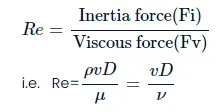
Here by changing the inlet velocity for different Reynolds number the flow can be captured
|
Reynolds number |
10 |
100 |
1000 |
10000 |
1 lakh |
|
Inlet Velocity |
0.15 |
1.5 |
15 |
150 |
1500 |
Solution:
Before giving the iterations we should make some checks for the results purpose. Creating a monitor point, lift force, drag force, velocity contour, pressure contour, vortex average for velocity, etc. These are given in the reports tab in Ansys fluent workbench setup command. Initialize the setup the animation for the velocity to check hoe the flow is behaves around this cylinder. By providing the 1000 iterations below are the results obtained.
Results:
PART1
|
Re No |
100(Steady) |
100(Unsteady) |
|
Scaled residuals |
 |
 |
|
Cl |
 |
 |
|
Cd |
 |
 |
|
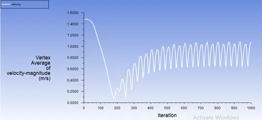
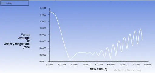
Velocity Magnitude |
 |
 |
|
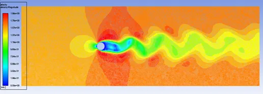
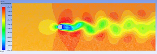
Velocity Contour |
 |
 |
|
Pressure Contour |
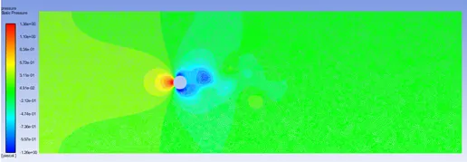 |
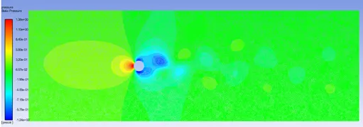 |
|
Strouhal No |
|
|
|
Velocity v/s Distance |
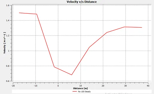 |
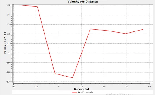 |
|
Velocity Animation |
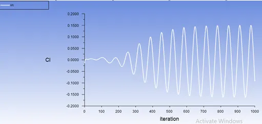
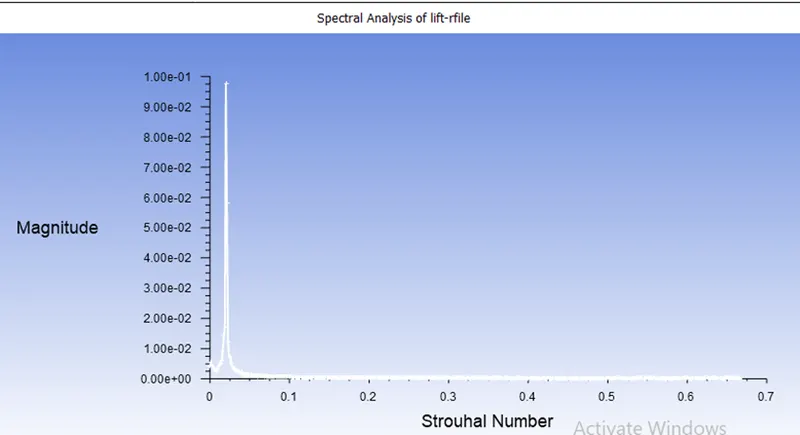
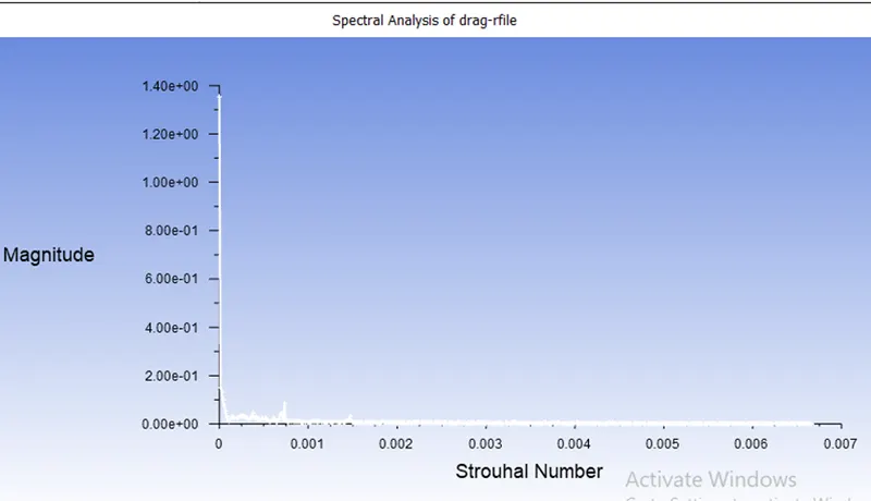
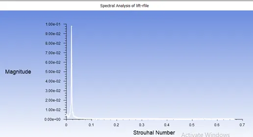 Max Lift=9.75e-02 St no=0.020
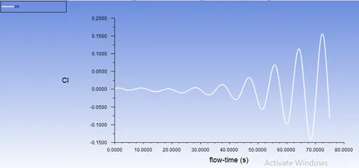
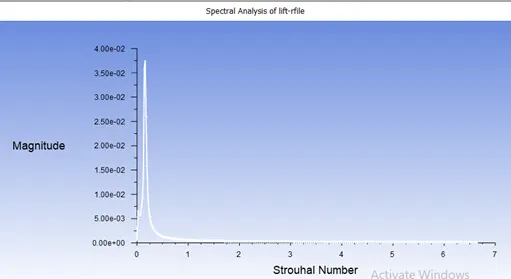 Max Lift=3.75e-02 St no=0.018
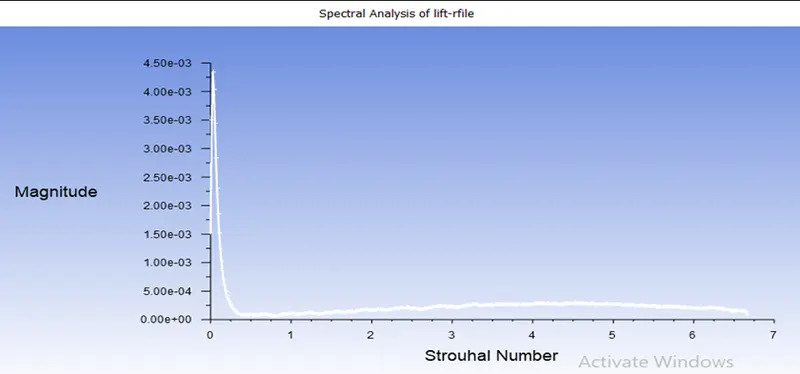
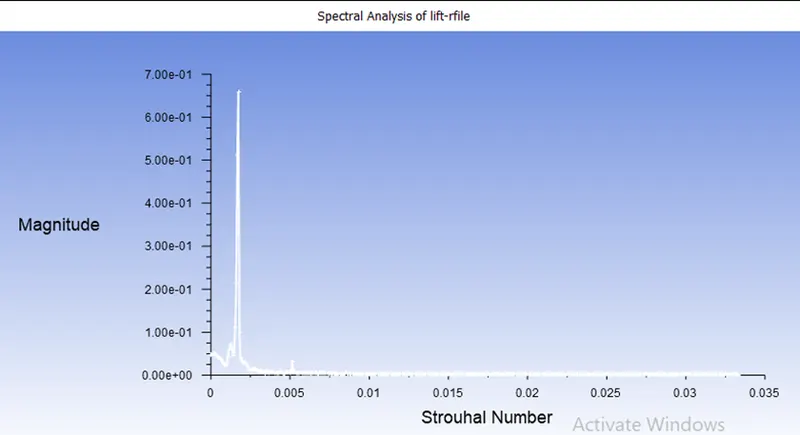
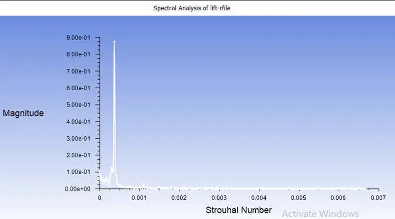
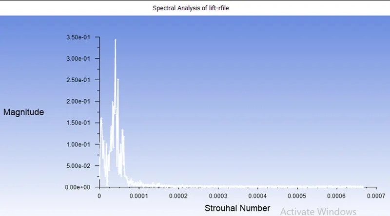
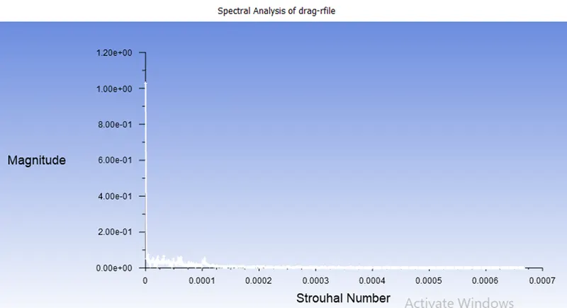
Strouhal Number:
The Strouhal Number represents a measure of the ratio of the inertial forces due to the unsteadiness of the flow or local acceleration to the inertial forces due to changes in velocity from one point to another in the flow field.
|
Re No |
Inlet velocity |
Cl |
Cd |
Monitor Velocity (m/s) |
Strouhal Number:
|
|
100(Steady) |
1.5 |
-0.092 |
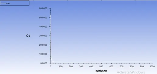
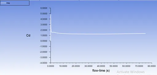
1.36 |
1.078 |
0.020 |
|
100(Unsteady) |
1.5 |
-0.081 |
1.35 |
0.635 |
0.018 |
PART2
Scaled residuals
|
Re No |
|
|
10 |
 |
|
100 |
 |
|
1000 |
 |
|
10000 |
 |
|
1 lakh |
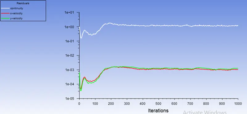 |
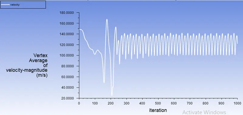
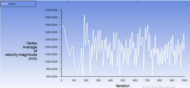
By observing the above residual plots after particular iterations the flow has converged means the flow gets steady there is no changes in the flow velocity in x,y direction, and continuity equations are also gets steady nature.
|
Re No |
Cl |
|
10 |
 |
|
100 |
 |
|
1000 |
 |
|
10000 |
 |
|
1 lakh |
 |
|
Re No |
Cd |
|
10 |
 |
|
100 |
 |
|
1000 |
 |
|
10000 |
 |
|
1 lakh |
 |
|
Re No |
Velocity Magnitude |
|
10 |
 |
|
100 |
 |
|
1000 |
 |
|
10000 |
 |
|
1 lakh |
 |
|
Re No |
Inlet velocity (m/s) |
Cl |
Cd |
Monitor Velocity (m/s) |
|
10 |
0.15 |
-0.0003 |
3.33 |
0.063 |
|
100(Steady) |
1.5 |
-0.092 |
1.36 |
1.078 |
|
100(Unsteady) |
1.5 |
-0.081 |
1.35 |
0.635 |
|
1000 |
15 |
-0.912 |
1.22 |
13.35 |
|
10000 |
150 |
0.378 |
1.46 |
121.92 |
|
1lakh |
1500 |
0.041 |
1.20 |
1148.75 |
|
Re No |
Velocity contour |
|
10 |
 |
|
100 |
 |
|
1000 |
 |
|
10000 |
 |
|
1 lakh |
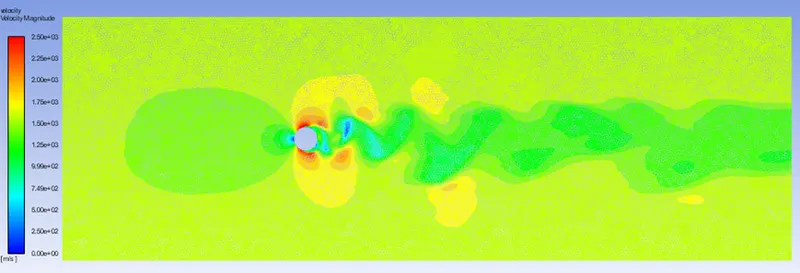 |
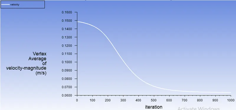
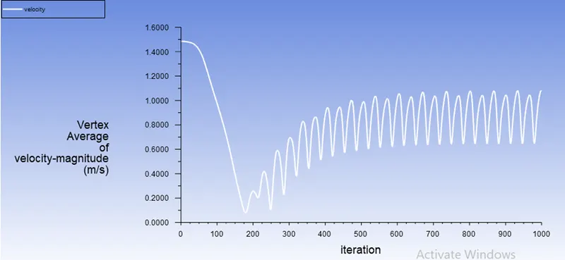
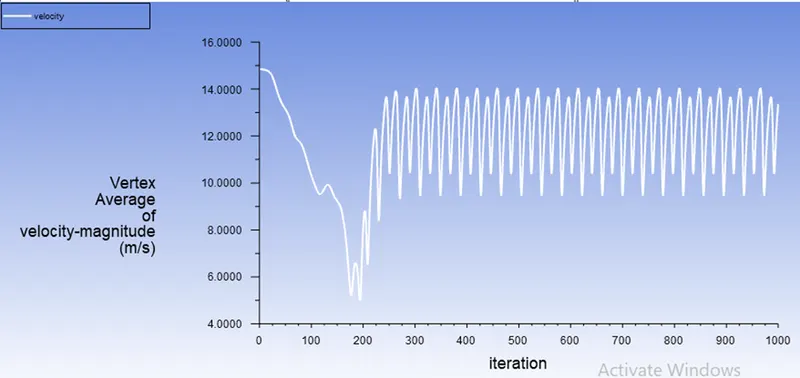
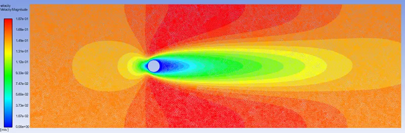
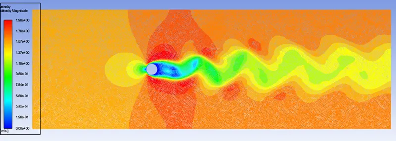
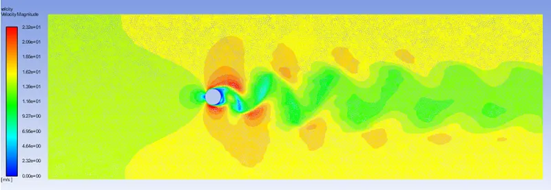
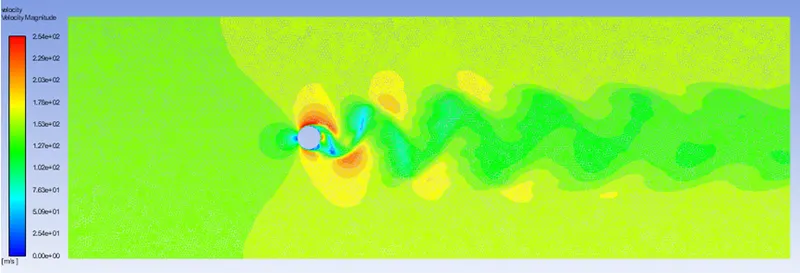
By observing the above velocity graphs we can conclude that for low Reynolds number the flow was laminar. By keeping the density constant and varying the viscosity and velocity the for Re 100 the flow was converting from laminar to transient flow and for higher Reynolds i.e. Re 1 lakh the flow is fully turbulent.
|
Re No |
Pressure contour |
|
10 |
 |
|
100 |
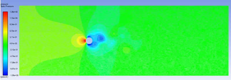 |
|
1000 |
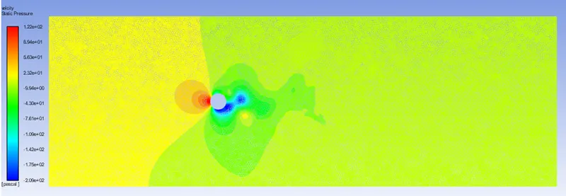 |
|
10000 |
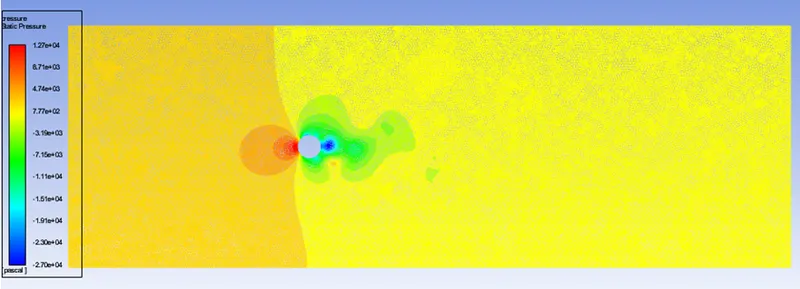 |
|
1 lakh |
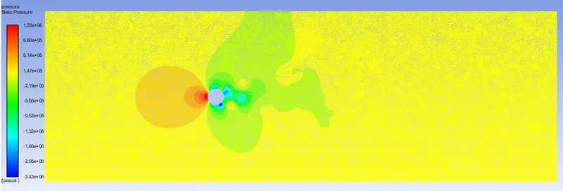 |
Strouhal Number:
|
Re No |
lift |
|
10 |
 |
|
100 |
 |
|
1000 |
 |
|
10000 |
 |
|
1 lakh |
 |
|
Re No |
Drag |
|
10 |
 |
|
100 |
 |
|
1000 |
 |
|
10000 |
 |
|
1 lakh |
 |
|
Re No |
Velocity v/s Distance |
|
10 |
 |
|
100 |
 |
|
1000 |
 |
|
10000 |
 |
|
1 lakh |
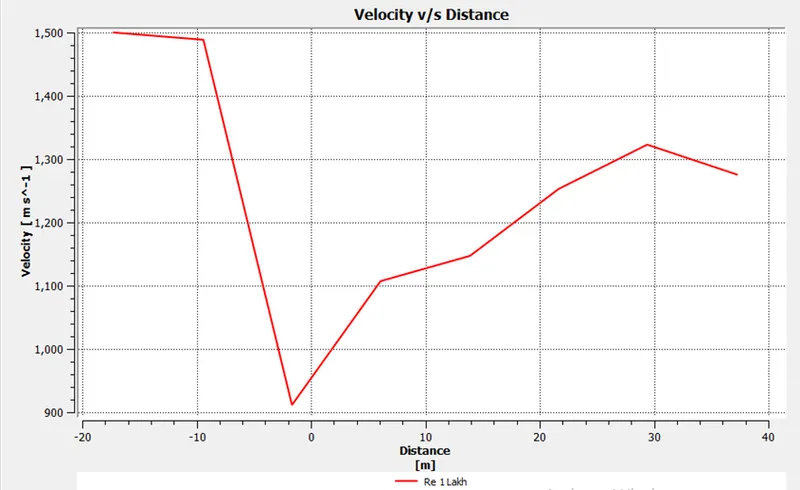 |
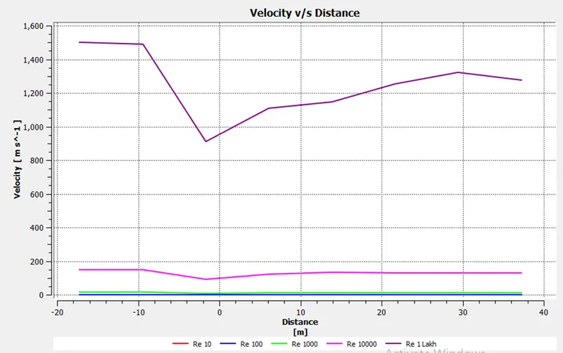
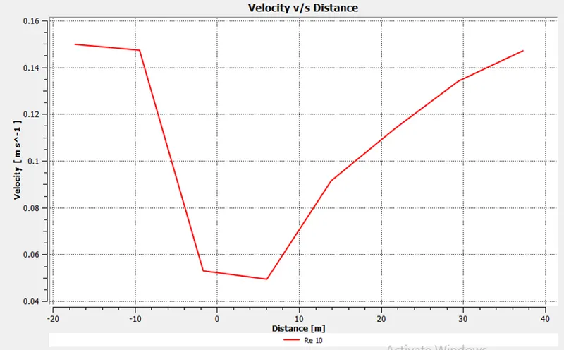
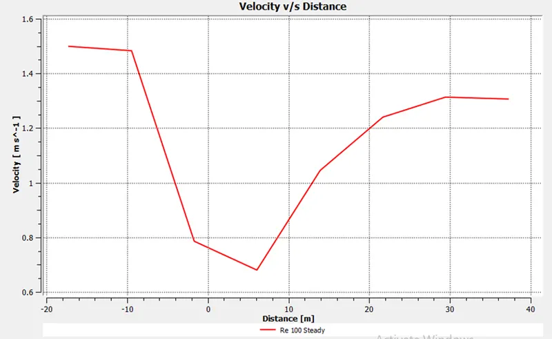
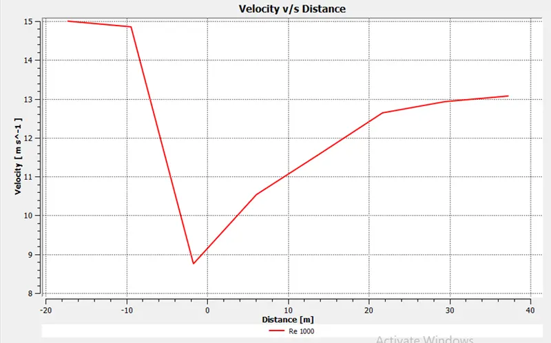
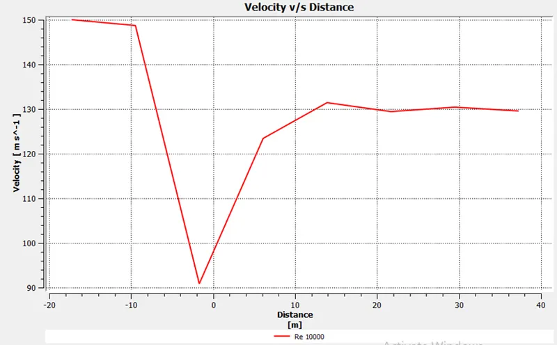
The above graph represents that for the low Re number i.e. 10 to 1000 the velocity is almost zero and it doesn’t varies along the distance , but when compare to the higher Re no10000 the velocity varies near the cylinder wall, in Re 1 lakh the velocity drastically varies near the cylinder wall and this is because of turbulent nature and the vortex shedding happens near the walls.
|
|
|
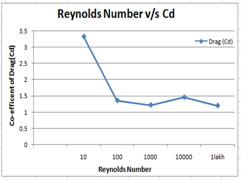 By Analysis
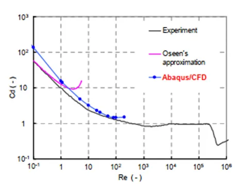 By Reference Paper
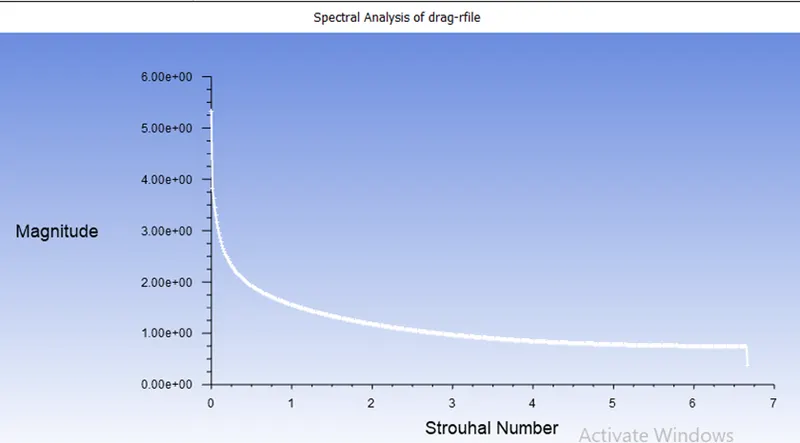
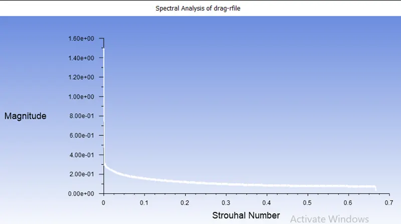
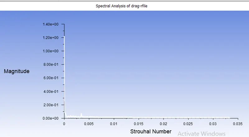
From the above graph it concludes that as the Reynolds number increases the coefficient of drag decreases and the results are identical from the reference paper.
|
Re No |
Velocity Animation |
|
10 |
|
|
100 |
|
|
1000 |
|
|
10000 |
|
|
1 lakh |
Result & Conclusion:
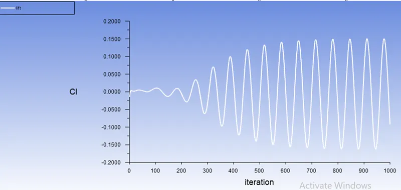
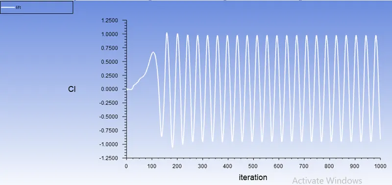
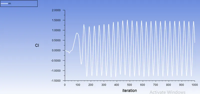
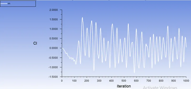
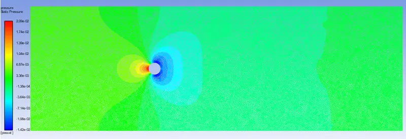
Using a 4 core CPU, the analysis has been performed. Streamlines are derived from the analysis and are shown in the above respected slots. For Re no 10 the streamlines are symmetrical. But For Re 100 and 1000 the streamlines are disturbed and are converting from laminar to transient condition and vertex shedding is started. For Re 10000 and one lakh condition the flow is fully turbulent and vertex shedding is distributed all over the front side of cylinder. The lift coefficient gradually increases as the Reynolds number increases, and the drag coefficient decreases as the Reynolds number increases.
Reference Research Paper:- https://imechanica.org/files/Sato_MDAC_final_2232012.pdf