Week 2 - Flow over a Cylinder.

Aim- introduction to GUI based CFD using Ansys, week_2 challenge flow over the cylinder.

Introduction- the part of the ANSYS by using ANSYS geometry we are creating a cylinder of some diameter and the surface around the cylinder for the fluid inlet and outlet, by providing some customized material in the inlet what kind of change is occurring in the fluid nature because of the cylinder in the path can be observed here.

We are using our own material having a limit set of Reynold number between 10 to 100, by changing the density and the viscosity of the fluid we will have the different type of fluid material and how the fluid trajectory and its properties are being changed because of the cylinder in the path can be seen by the help of ANSYS fluent.

Theory- here we are going to perform the 2-D simulation by modifying the Reynold number by customizing our own fluid by changing its property for this we are also going to create the run time analysis for the steady and transient flow. Visualizing the vortex shedding by adding motion points.

Procedure of modelling approach with the solver setting -

Step -1 launch the workbench drag fluent workbench > open geometry space clan> name it flow over the cylinder> set unit under the file unit and meter for the length.

Now we are going to create a circle of 2 m and from the centre 10D =20m left and 20D= 40m to the right having 10D of width there will be a rectangular. Now use pull to make it as a surface, delete all the line and circle edge. Close the geometry and update the mesh.

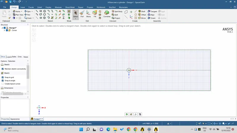
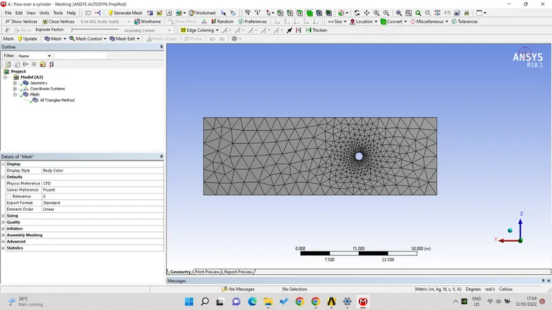
Step -2- here the mesh is having the quadrilateral mesh element geometry, Add< method< geometry select the face( all the selected face will have the blue color)> select triangle> sizing of the mesh element< 2m.

Select the edge of the circle<no of division 36 ( as the circle having 360 degree and the 10 division will be enough ) click ok the generated mesh will be much smooth.

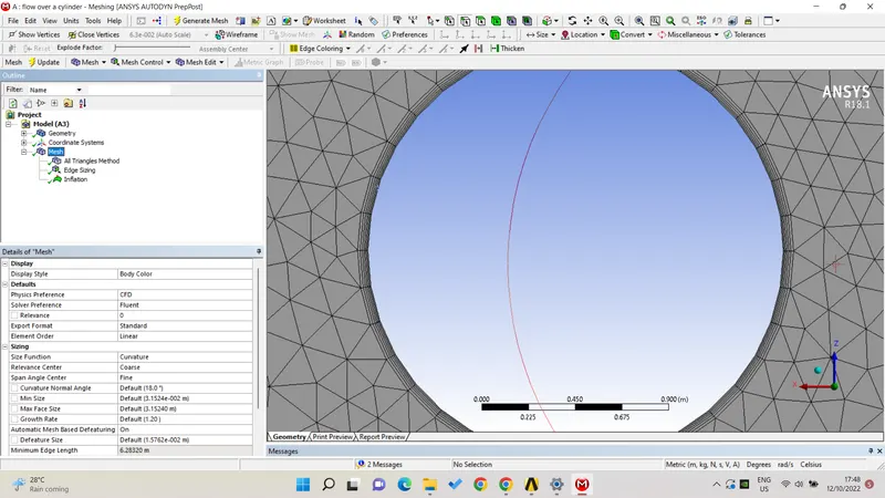
Now we are going to add the inflation layer ( it helps in creating the fitted body as in case of CAD file) < select body <under boundary < select the edge of circle>5e-3 thickness< no of layer is6( this is enough<here the growth rate is 1.2 as the 20% with each layer.

Name all boundary as left side is inlet, right side is outlet, wall and symmetry.

Step-3 setup the physics, steady state ( constant with the time) pressure based > velocity absolute< viscosity< laminar ( because the Reynold number.

Material < fluent database < new< give the density to 1 kg/m3 and the viscosity to the 0.05kg/m-s< change/ create< close< delete all the remain unwanted material. Here the fluent is take the air as the default material, we need to change this< cell zone< fff- surface<9 defines volume)<edit< material< select the user material<ok.

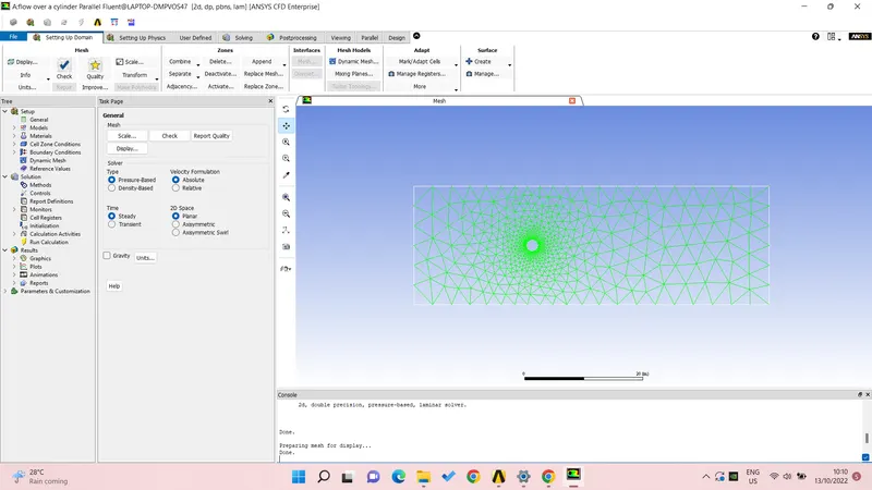
Now see the boundaries.

Inlet< velocity inlet< 1m/s

Outlet<pressure head< 0 pascal (gauge pressure is zero thus here the atm pressure is there which is 1 atm)

Wall< no slip<boundary condition for the cylinder

Solving > definition> new> area> vortex average>need to give the monitor point here for this again go to the post processing > insert> point> x is 4D= 8m< y is zero< name it as a monitor point< create it will show on the right side from the cylinder.> select the variable to the velocity< velocity magnitude<select the monitor point<< report file< report plot < frequency 1.

Make the hybrid initialization.

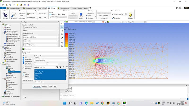
Post process>contour> new>name it as velocity. Filled option> select all from the table> save> display< commute the hybrid initialize.

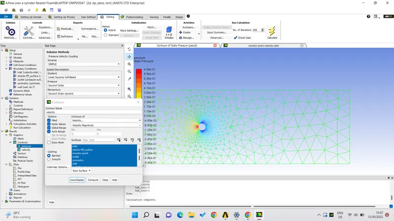
New contour < pressure< select pressure<filled< select all the option from table<save and display> compute the initial hybrid initialize.

Step-4 the method will be simple here, uncheck the residual convergence area criteria hereselect the iteration 350 and calculate.

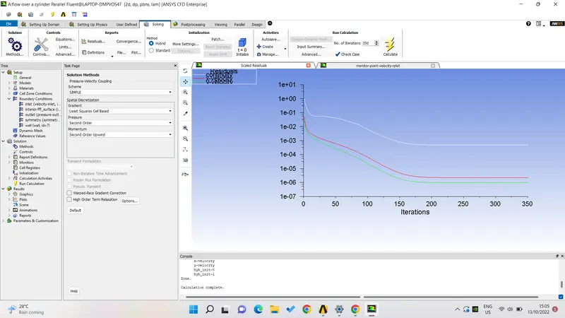
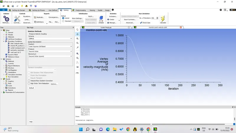
Here to see the result more on accurately we are going to add the animation here> activity>create>solution animation>name it as the velocity animation>make it record it after every 10iteration> select velocity. Now in the table of content we can see under the animation there is the name under velocity animation now give the iteration again some value and make it calculate.

Result- here the result is not good we are not able to see the changes in the pressure at the outlet and the velocity at the monitor point very accurately , thus we are going to rife our result by providing more fine mesh, this time going to take the mesh length is 1m , for this again going in the mesh change the element size to 1m generate the mesh update the mesh then again come in the setup check for the material and initialize the result( it will delete the preprocessing)

As in this case also the result is not matching our expectation thus we are asking again the mesh element size to 0.25 m and generating the mesh with again updating the setup, the mesh will something look like this.

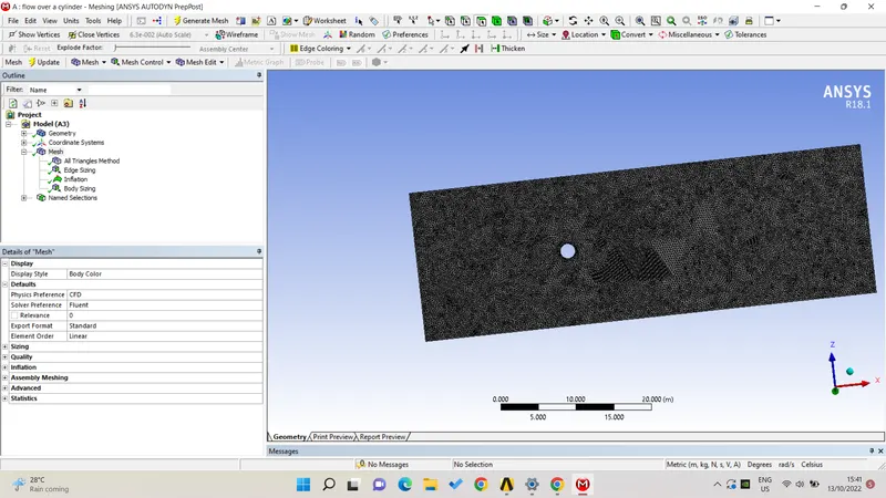
Now for the same material we will see the iteration and graph setting for the flow of our customized material.

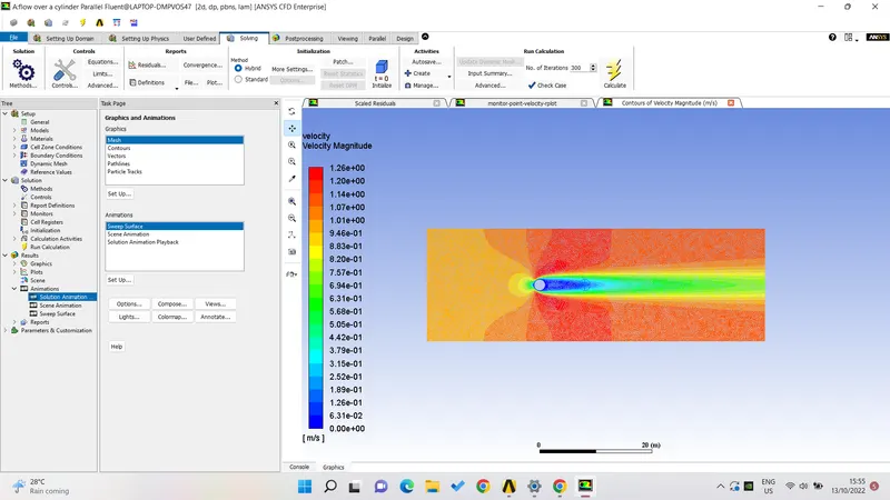
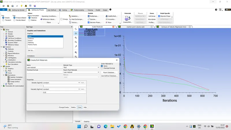
But now still we are not getting the vortex shedding at the outlet now we will change our viscosity value which we change our Reynold number to 40 and then 100 here I am attaching the result of 700 iteration with 0.045kg/m-s viscosity and 0.02 kg/ m-s

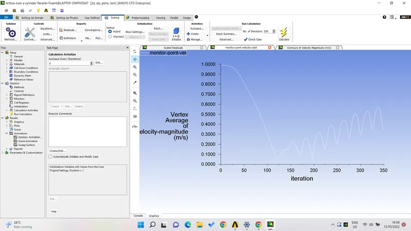
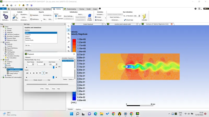
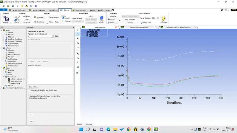
Here we can see the velocity is oscillating and some vortex is forming there at the monitor point to the exit of the flow it can also be seen over the plot that velocity is not reach to the steady state as it’s been changing at each point of time., this steady state analysis we do to see the end result only.

Thus at last we will do some transient steady as well for the same material having same Reynold number but the time step is 0.1 sec> and 500 time step it will run until some end result will not come.

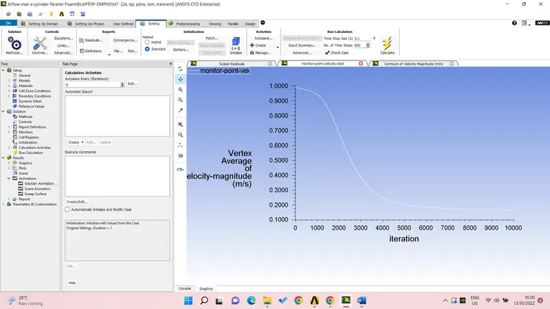
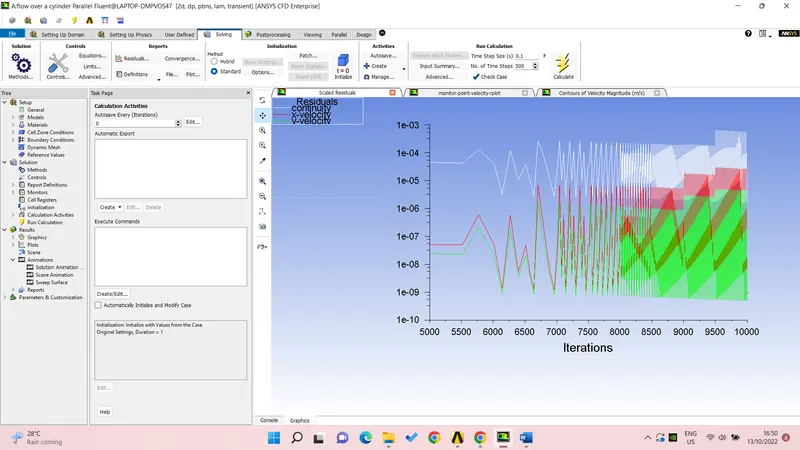
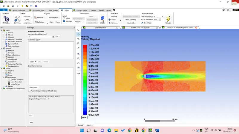
Here you can see the iteration is went up to 10k time to given some refined result.

Conclusion- ANSYS fluent is converting the mathematical equation of fluid to show some visual result, here our task or our end result is not only is to generate the colorful image but also we need to analysis them in case of different condition with different input condition as we didid here.

We have started with the not so refined mesh to come at the end with very refined mesh also by changing the property of our customized fluid at the inlet we have seen the various result with the von Karman vortex shedding for the laminar flow having Reynold number of 100.

Thus my task was to learn something from the challenge here and at the end as I made the detailed report for the challenge I can say I have provide my new learning in the ANSYS software.