Week 2 - Flow over a Cylinder.
AIM: To simulate the unsteady and steady-state flow over a cylinder using
INTRODUCTION: In fluid dynamics, vortex shedding is a turbulent flow that takes place when a fluid such as air or water
As flow past a body certain velocity, depending on the size and shape of the body the flow starting backward flow due to negative pressure behind the body. In this flow, vortices are created at the back of the body and detach periodically from either side of the body forming a Von Karman
vortex street which is responsible for the unsteady separation of the flow of a fluid around blunt bodies. It is named after the engineer and fluid dynamitist Theodore von Karman. The fluid flow past the object creates alternating low-pressure vortices on the downstream side of the object. The object will tend to move toward the low-pressure zone.
A vortex street will form only at a certain range of flow velocities, specified by a range of Reynolds numbers (Re), typically above a limiting Re value of about 100. The Reynolds number for a flow is a measure of the ratio of inertial to viscous forces in the flow of a fluid around a body or in a channel.
Methodology
- create 2D body in space claim
- create a mesh of 2d geometry of space
- define boundary condition
- define material properties as per study requirement
- set parameter to study flow simulation
flow simulation setup
- Geometry:
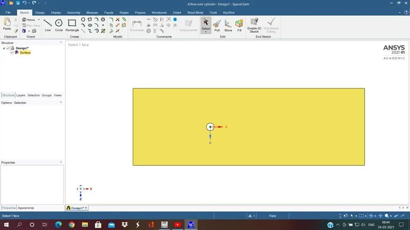
First, the cylinder boundary is to be drawn in the space claim and its dimensions
Cylinder diameter = 2.00M
Inlet boundary distance from cylinder wall = 10*2.00 M
Outlet boundary distance from cylinder wall = 20*2.00 M
Symmetry boundary distance from cylinder wall = 5*2.00 M
To make space for study pull Out and delete geometry construction line
2.Mesh:
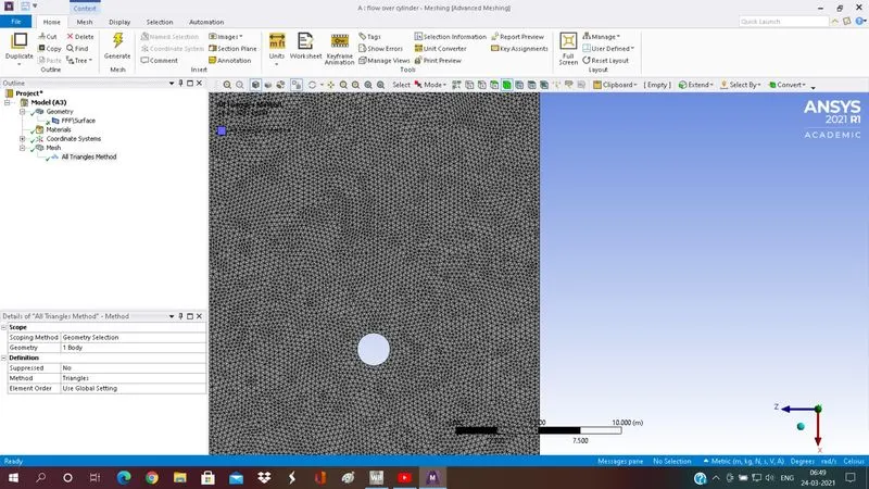
Generate mesh with the default setting
Meshing element type All triangular method
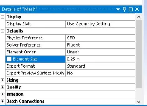
After add the meshing sizing method
Mesh sizing = 0.25M
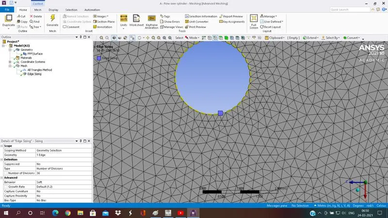
Add inflation method for cylinder wall
First layer thickness 5e-3
With incremental factor 1.2
inflation layers are 6 nos’
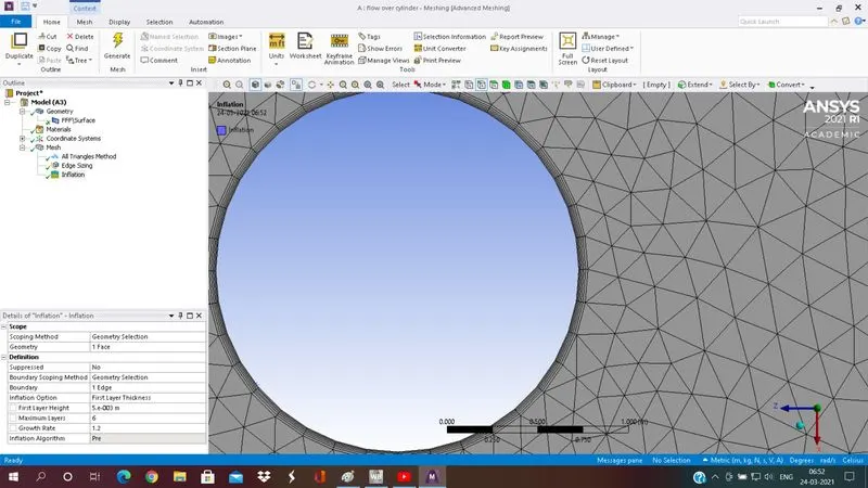
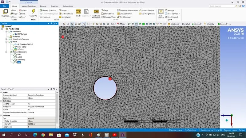
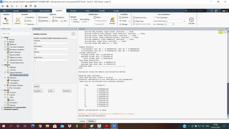
- fluent setup
General solver setup
- Steady-State Simulation
- Pressure based solver
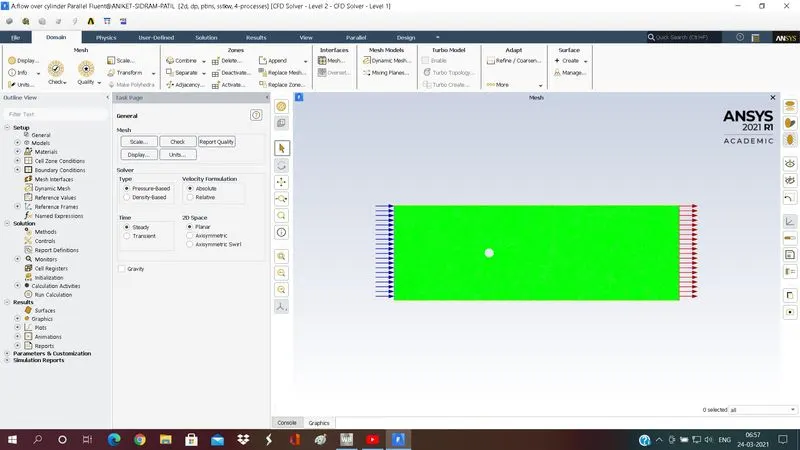
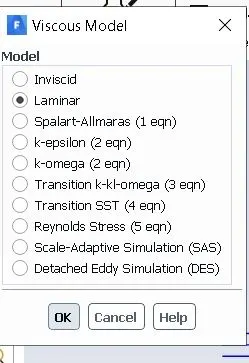
Viscous model
- laminar
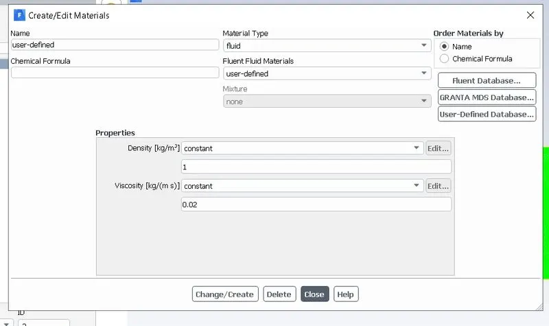
Set material properties – user-defined
- density = 1
- viscosity = 0.02
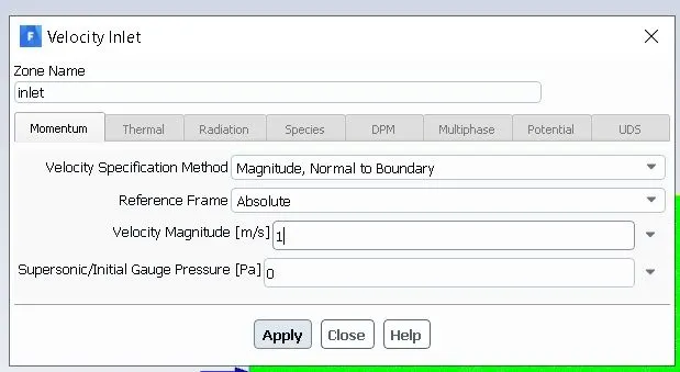
Boundary condition
- Inlet velocity = 1 m/s
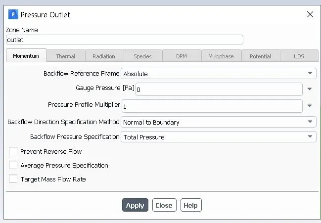
- Outlet
Pressure = default
Gauge pressure = 0
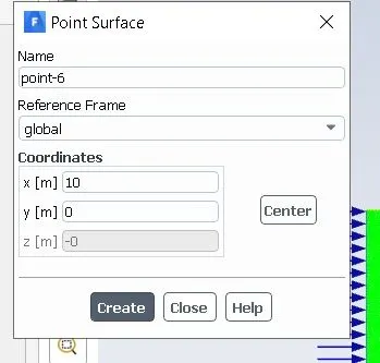
Generate point
- Monitor point
X= 10
Y= 0
Initialize hybrid method
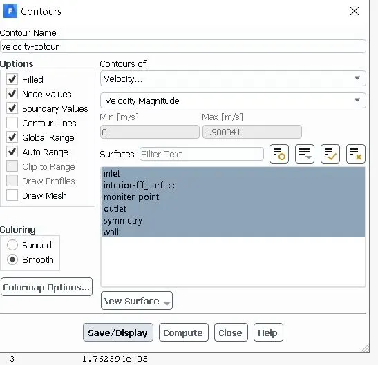
Velocity contour
- Select all surfaces
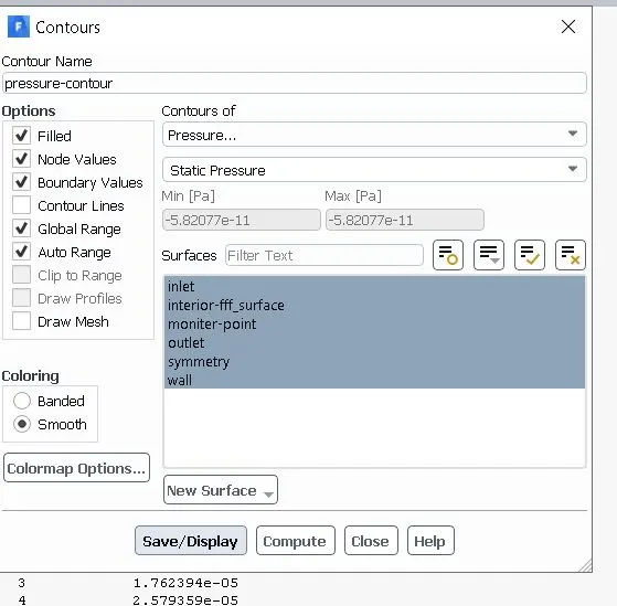
Pressure contour
- Select all surfaces
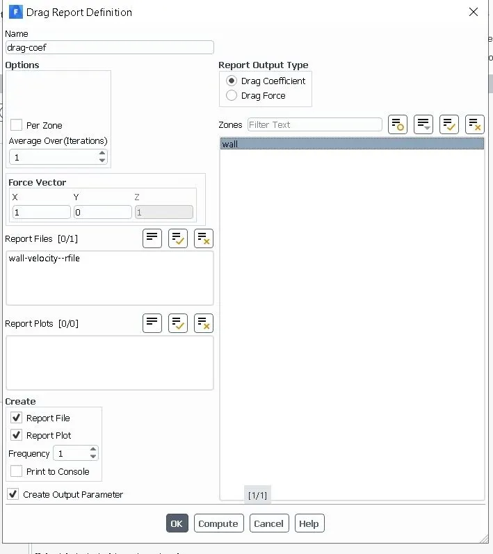
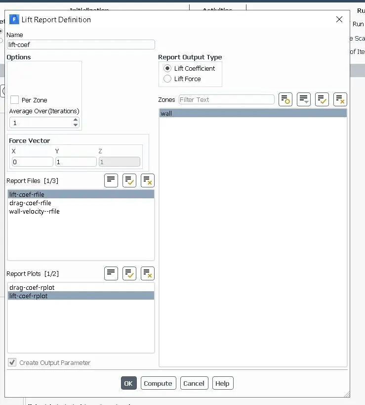
New force report
- Drag coefficient
- Lift coefficient
Initialize hybrid method
Results
Case-1: Steady-State For Re=10 where viscosity=0.02 and velocity=0.1m/s
for 500 Otration
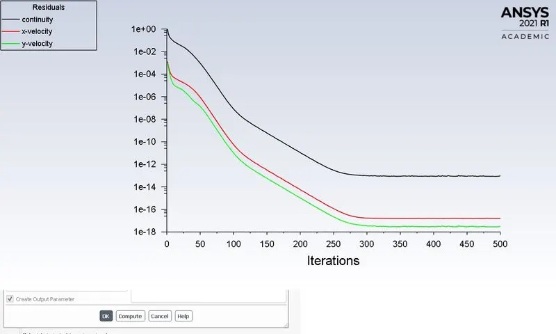
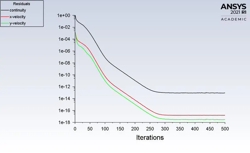
1. Residual plot:
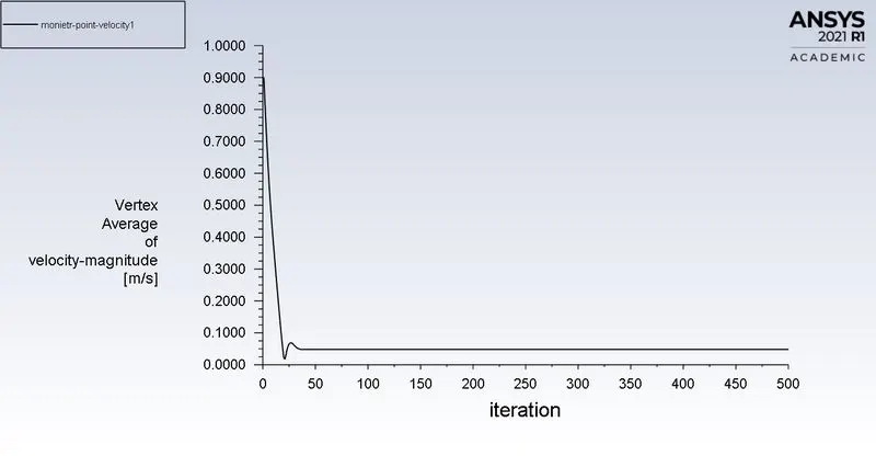
2. Monitor point velocity:
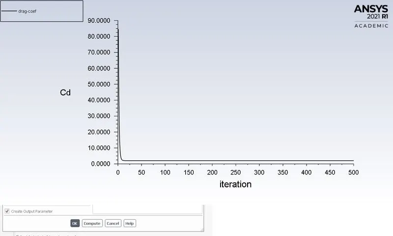
3.Drag coefficient:
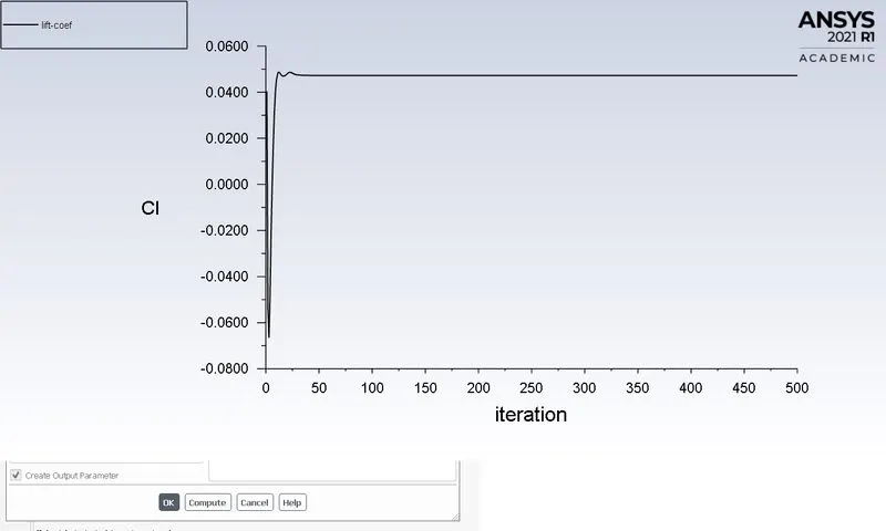
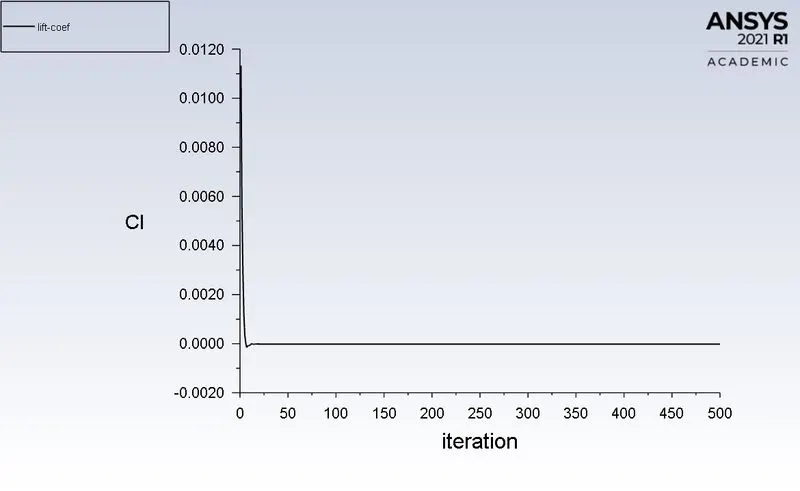
4. Lift coefficient:
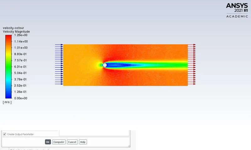
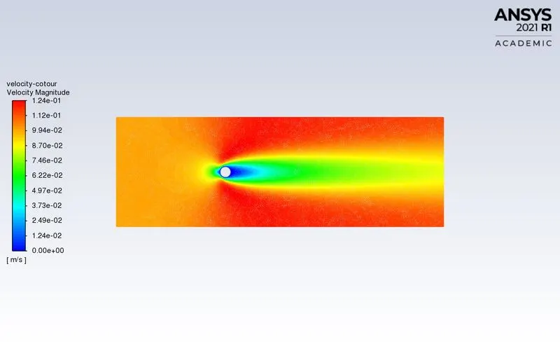
5.velocity contour:
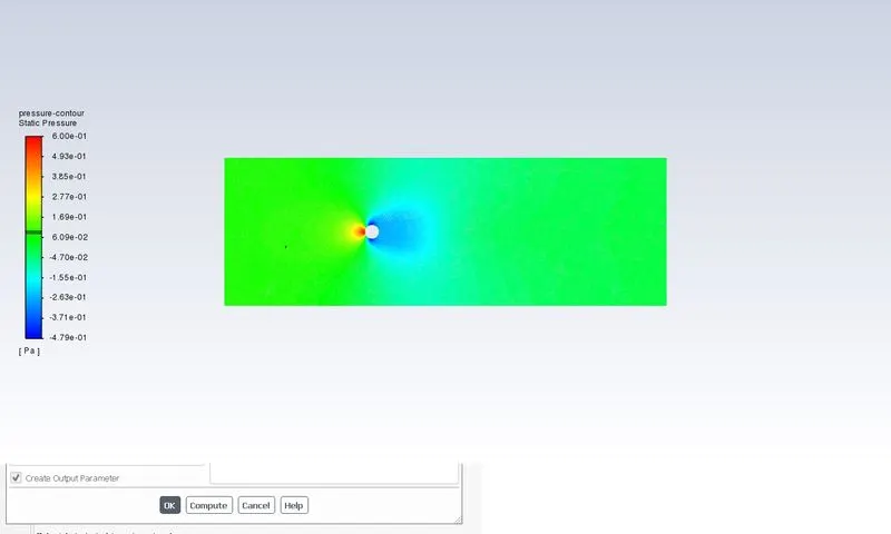
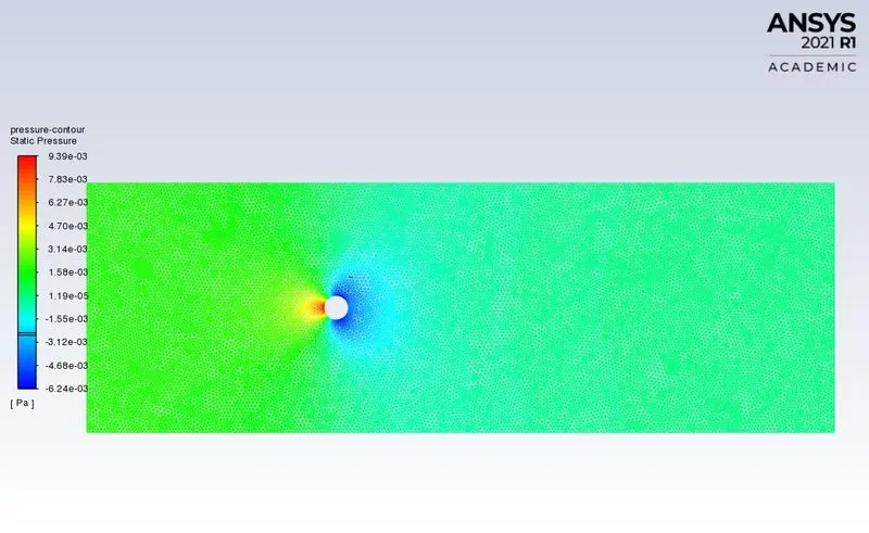
6. Pressure contour
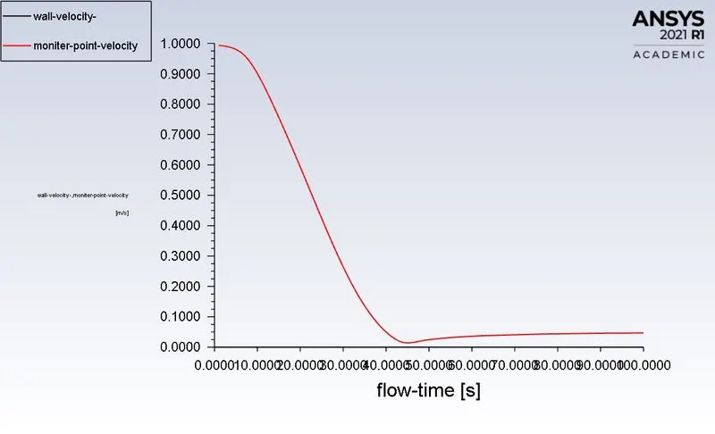
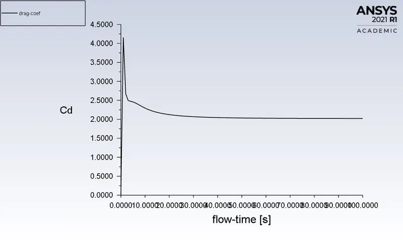
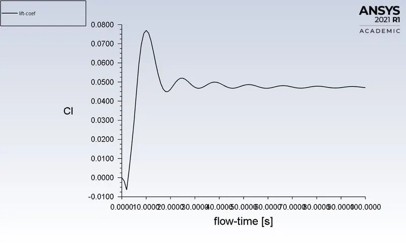
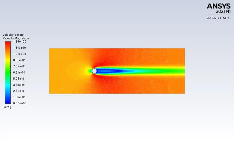
Case 2: Unsteady State ( Transient )
For Re=10 where viscosity=0.02 and velocity=0.1m/s
for 100 no. of time factor
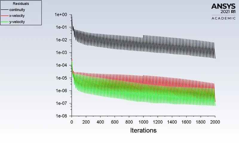
1. Residual plot:
2. Monitor point velocity:
3.Drag coefficient:
4. Lift coefficient:
5.velocity contour:
6. Pressure contour
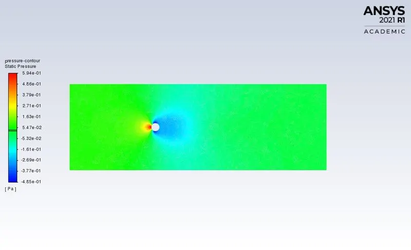
Case-3 : For Re=10 where viscosity=0.02 and velocity=0.1m/s
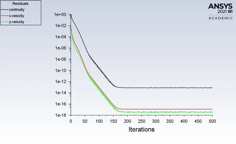
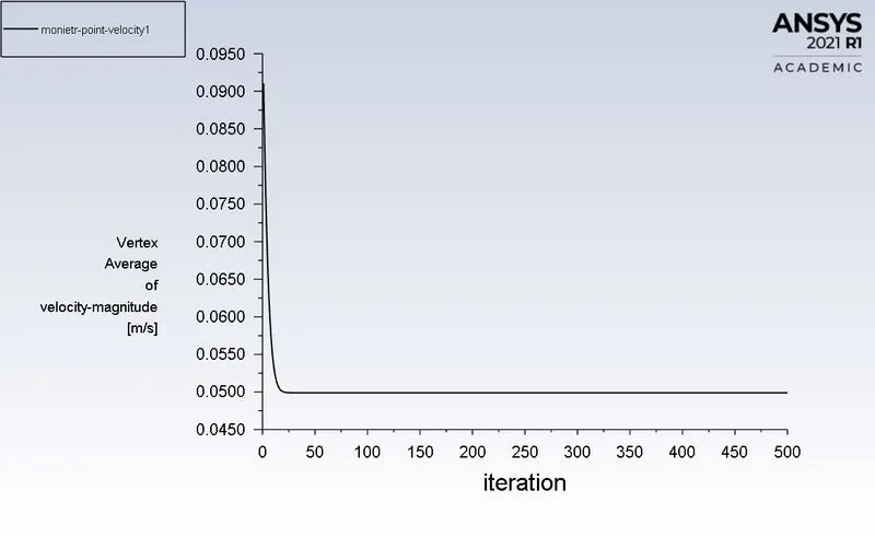
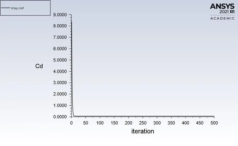
no. of iteration 500
1. Residual plot:
2. Monitor point velocity:
3.Drag coefficient:
4. Lift coefficient:
5.velocity contour:
6. Pressure contour :
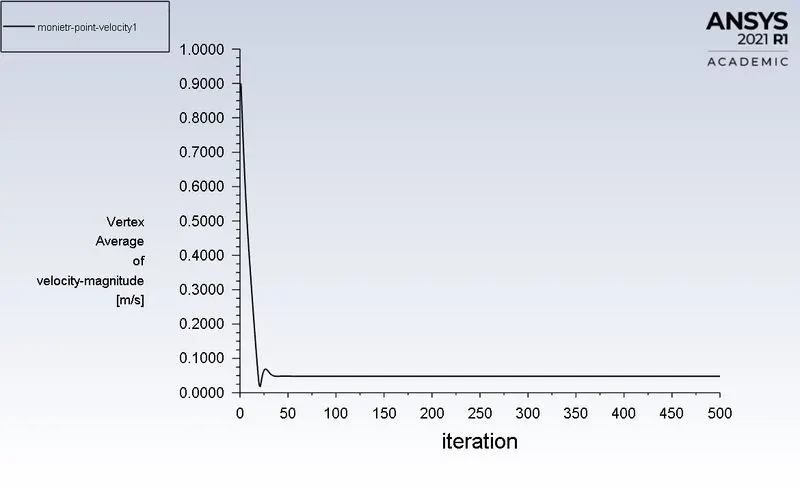
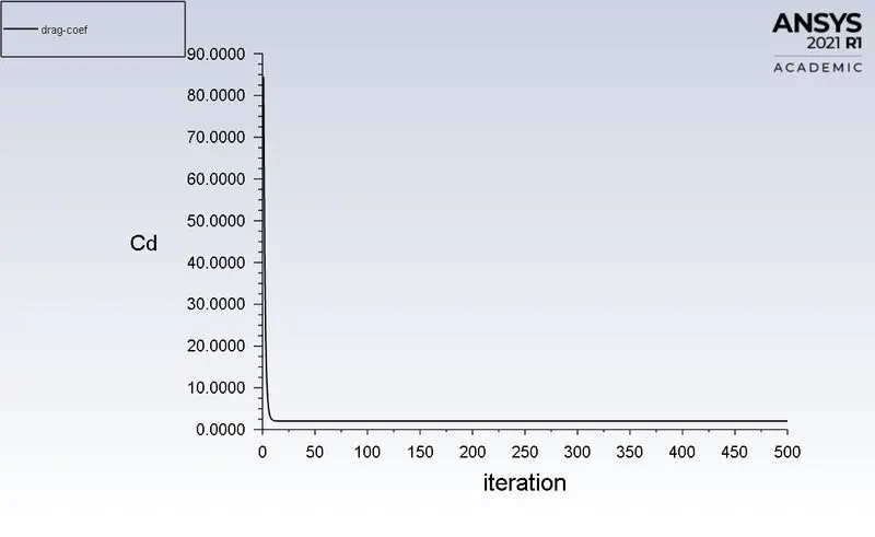
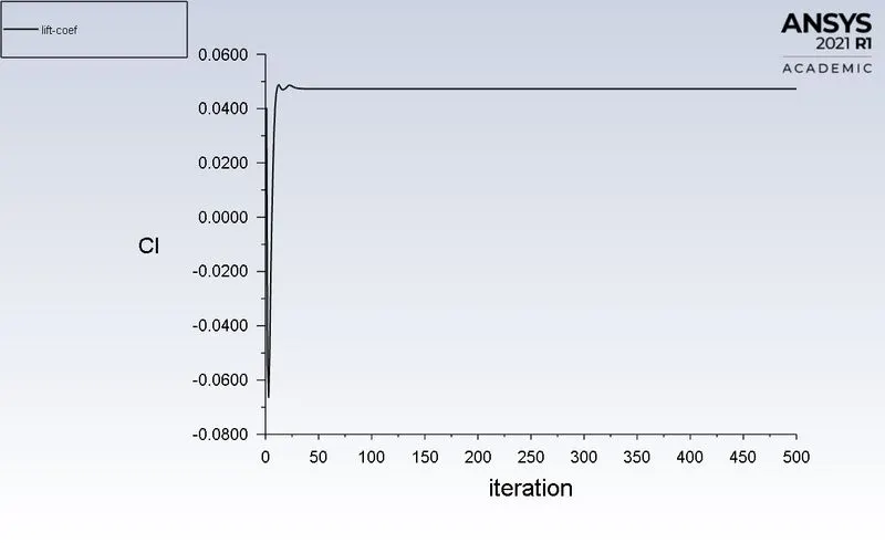
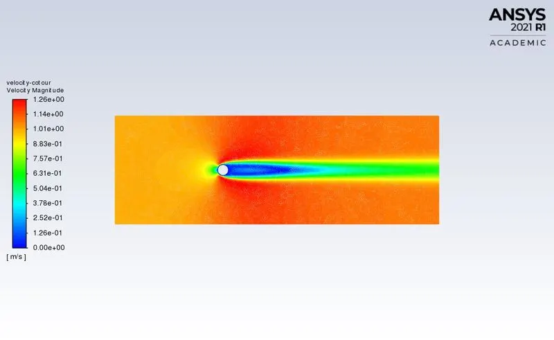
Case-4 : For Re=100 where viscosity=0.02 and velocity=1m/s
1. Residual plot:
2. Monitor point velocity:
3.Drag coefficient:
4. Lift coefficient:
5.velocity contour:
6. Pressure contour :
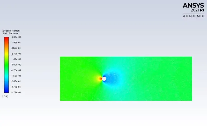
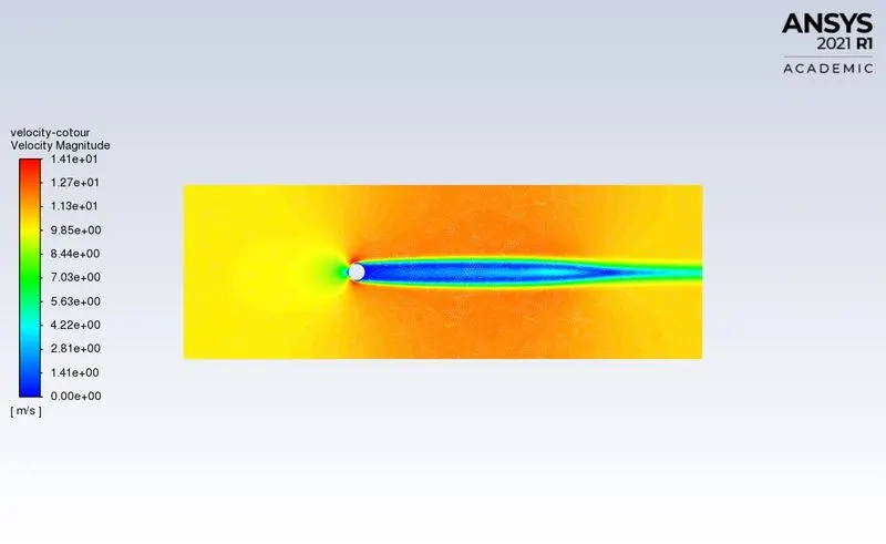
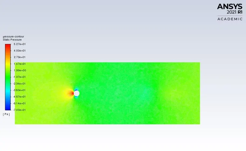
Case-5 : For Re=1000 where viscosity=0.02 and velocity=10m/s
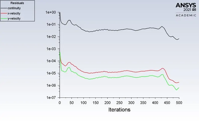
1. Residual plot:
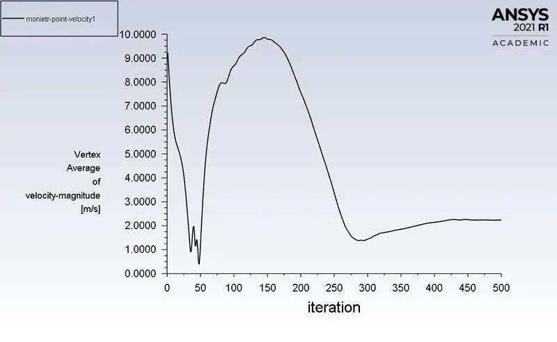
2. Monitor point velocity:
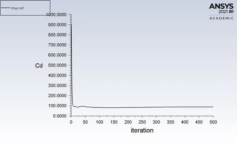
3.Drag coefficient:
4. Lift coefficient:
5.velocity contour:
6. Pressure contour :
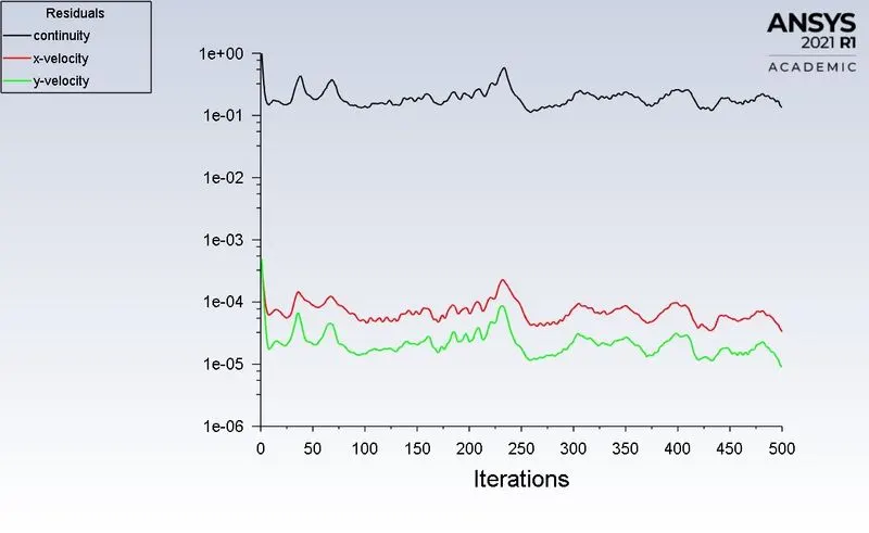
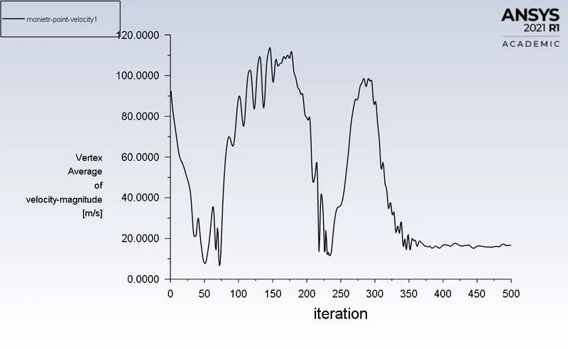
Case-6: For Re=10000 where viscosity=0.02 and velocity=100m/s
1. Residual plot:
2. Monitor point velocity:
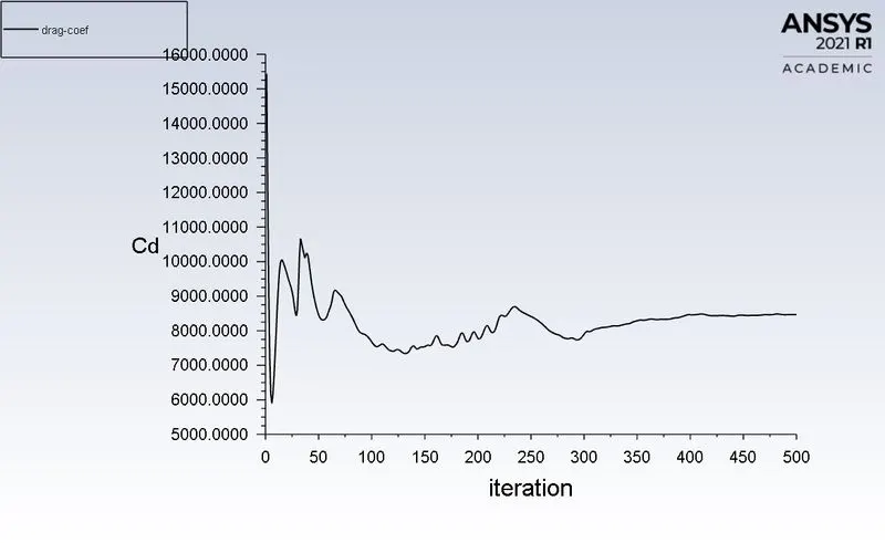
3.Drag coefficient:
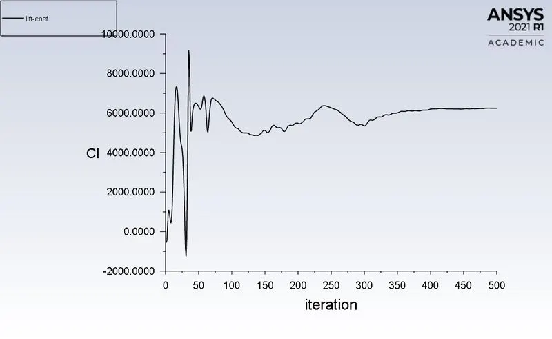
4. Lift coefficient:
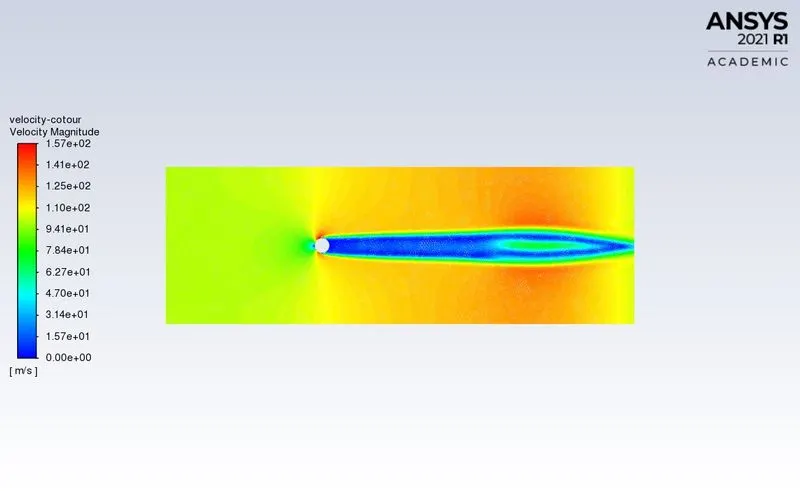
5.velocity contour:
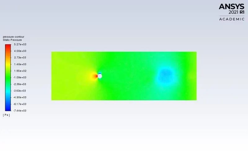
6. Pressure contour :
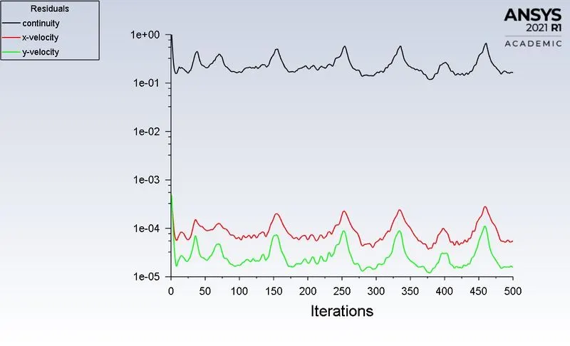
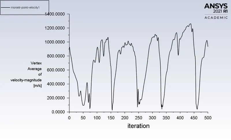
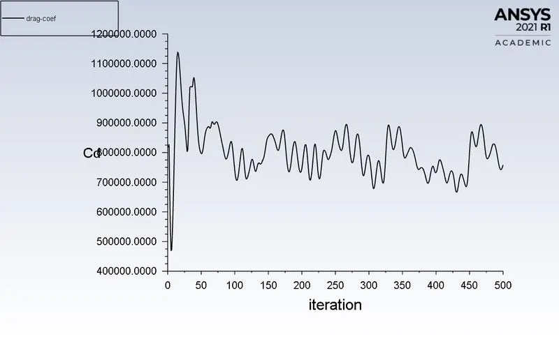
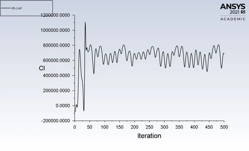
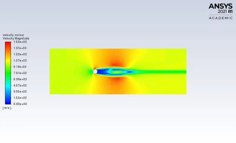
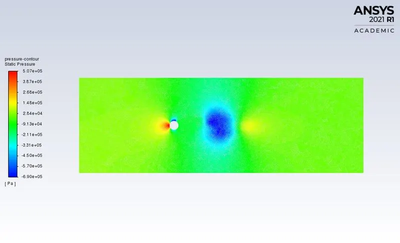
Case-7: For Re=100000 where viscosity=0.02 and velocity=1000m/s
1. Residual plot:
2. Monitor point velocity:
3.Drag coefficient:
4. Lift coefficient:
5.velocity contour:
6. Pressure contour :
observation :
1. to study the effect of Reynolds no. on flow over cylinder the flow simulation on Ansys fluent is carried out with increasing no. of inlet velocity with a constant fluid density as shown above.
2.in this flow simulation all the data has been plot with respective Reynolds no. like scaled residual, monitor point velocity, drag and lift coefficient on the body, velocity, and pressure contour plot record simultaneous changes in vortex shedding behind the body
3. As the fluid velocity increases over the Reynolds no. the monitor point velocity plot shows cyclic graph over itration as the flow increases
4. As the Reynold no. increases the drag and lift coefficient acts more violently.
5. vortex shedding is observed as the velocity increases as we can see on scaled residual and moniter point velocity
Results :
1. Vortex shedding observed as the Reynolds no. increases with inlet velocity
2. cd And cl show changes in the plot as the Reynold no. increases
3. as the results are in laminar flow but showing results the flow is converting from laminar flow to turbulent flow, this simulation shows the flow transformation from laminar to turbulent flow.