Week 2 - Flow over a Cylinder.
AIM :- Simulate the flow over a cylinder and explain the phenomenon of Karman vortex street.
PART-I
1. Simulate the flow with the steady and unsteady case and calculate the Strouhal Number for Re= 100.
PART-II
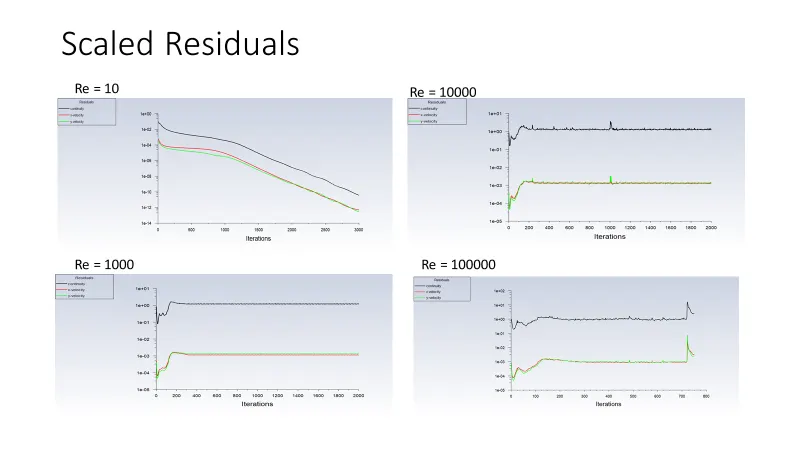
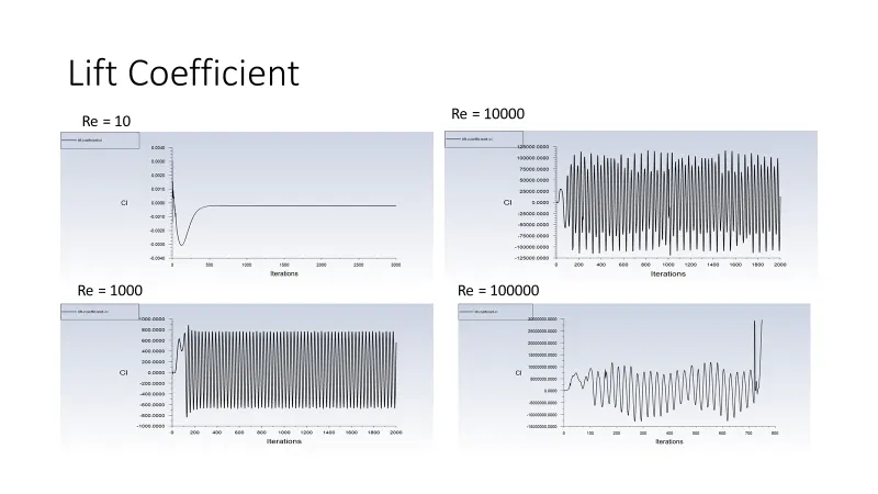
1. Calculate the coefficient of drag and lift over a cylinder by setting the Reynolds number to 10,100,1000,10000 & 100000. (Run with steady solver)
2. Discuss the effect of Reynolds number on the coefficient of drag.
INTRODUCTION :-
In fluid dynamics, a Kármán vortex street (or a von Kármán vortex street) is a repeating pattern of swirling vortices, caused by a process known as vortex shedding, which is responsible for the unsteady separation of flow of a fluid around blunt bodies.
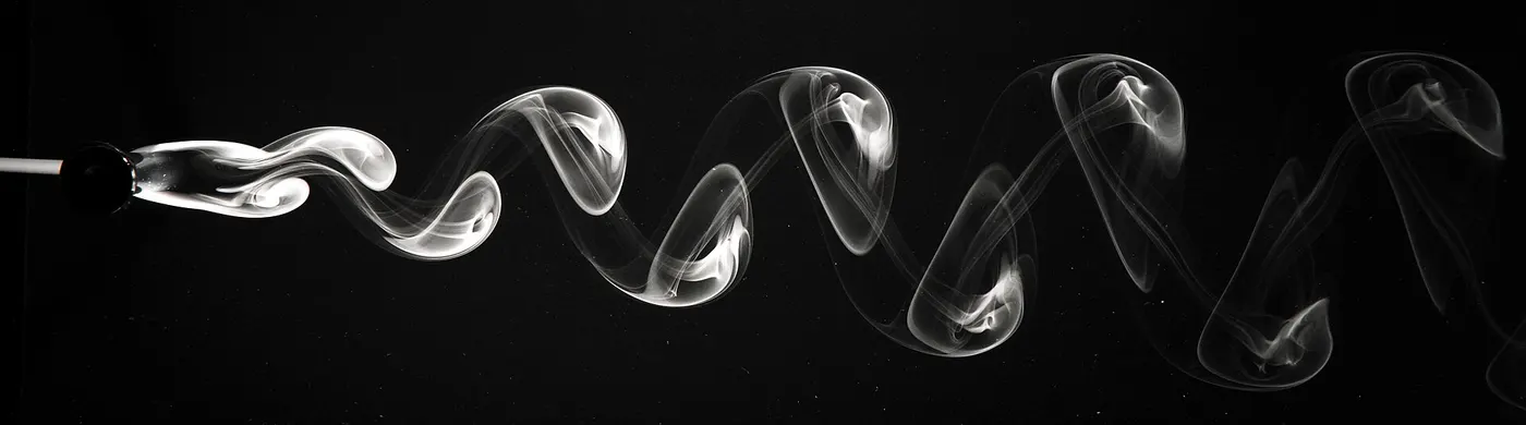
Visualisationof the vortex street behind a circular cylinder.
KARMAN VORTEX STREET :-
A vortex street will form only at a certain range of flow velocities, specified by a range of Reynolds Number (Re), typically above a limiting Re value of about 90.
The (global) Reynolds number for a flow is a measure of the ratio of inertial to viscous forces in the flow of a fluid around a body or in a channel, and may be defined as a nondimensional parameter of the global speed of the whole fluid flow.
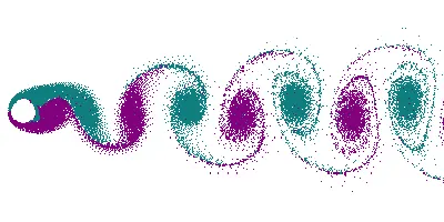
Animation of vortex street created by cylindrical object
The Reynolds number for a flow is a measure of the ratio of inertial to viscous forces given by
Re = ( [ ρ*u*D ] / μ )
where
ρ = Density of fluid ---> Kg/m^3
u = Flow Speed ----> m/s
D = Diameter of Cylinder ---> m
μ = Dynamic Viscosity ---> Kg/(m-s)
The range of Re values will vary with the size and shape of the body from which the eddies are being shed, as well as with the kinematic viscocity of the fluid.
Over a large Re range (47<Re<10 for circular cylinders; reference length is d: diameter of the circular cylinder) eddies are shed continuously from each side of the circle boundary, forming rows of vortices in its wake.
The alternation leads to the core of a vortex in one row being opposite the point midway between two
vortex cores in the other row, giving rise to the distinctive pattern. Ultimately, the energy of the vortices is consumed by viscosity as they move further down stream, and the regular pattern disappears.
When a single vortex is shed, an asymmetrical flow pattern forms around the body and changes the pressure distribution. This means that the alternate shedding of vortices can create periodical lateral (sideways) forces on the body in question, causing it to vibrate. If the vortex sheddingfrequency is similar to the natural frequency of a body or structure, it causes resonance.
VORTEX SHEDDING :-
In fluid dynamics, vortex shedding is an oscillating flow that takes place when a fluid such as air or water flows past a bluff (as opposed to streamlined) body at certain velocities, depending on the size and shape of the body.
In this flow, vortices are created at the back of the body and detach periodically from either side of the body forming a Karman vortex street.
The fluid flow past the object creates alternating low-pressure vortices on the downstream side of the object. The object will tend to move toward the low-pressure zone.
GOVERNING EQUATION :-
The frequency at which vortex takes place for an infinite cylinder is related to the Strouhal number by the following equation,
Sr = ( [f*D] / V )
Where,
f --> Vortex shedding frequency
D --> Diameter of the cylinder
V --> Flow velocity
PROCEDURE AND RESULTS
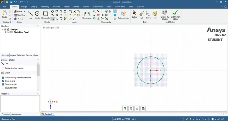
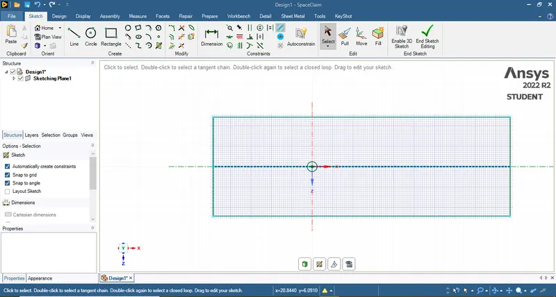
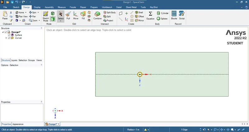
GEOMETRY
The Geometry has been provided in the challenge interface.
MESH GENERATION :-
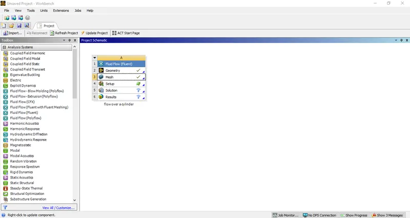
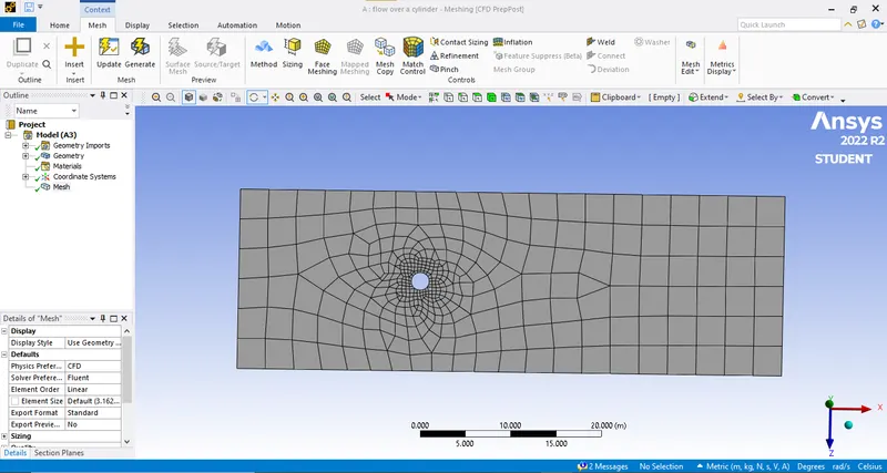
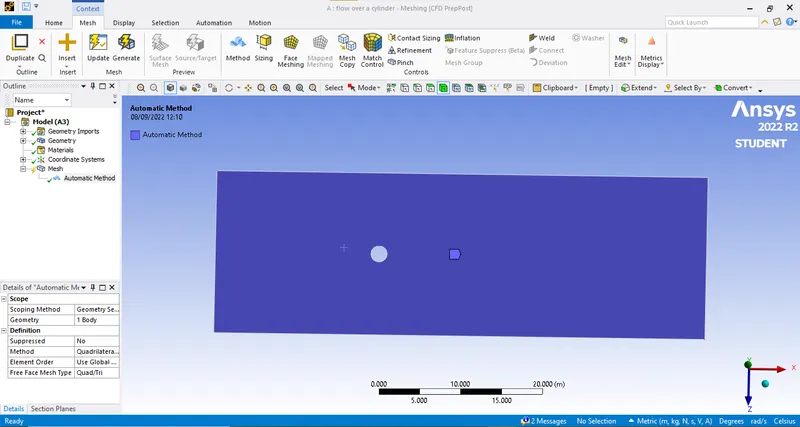
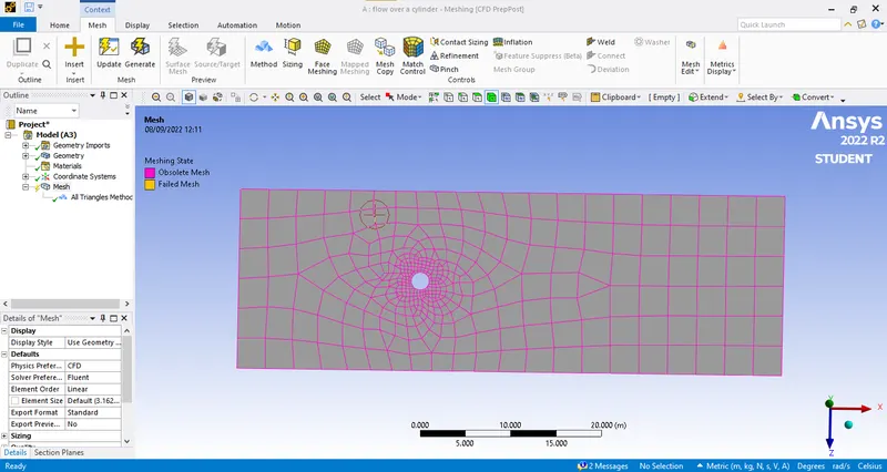
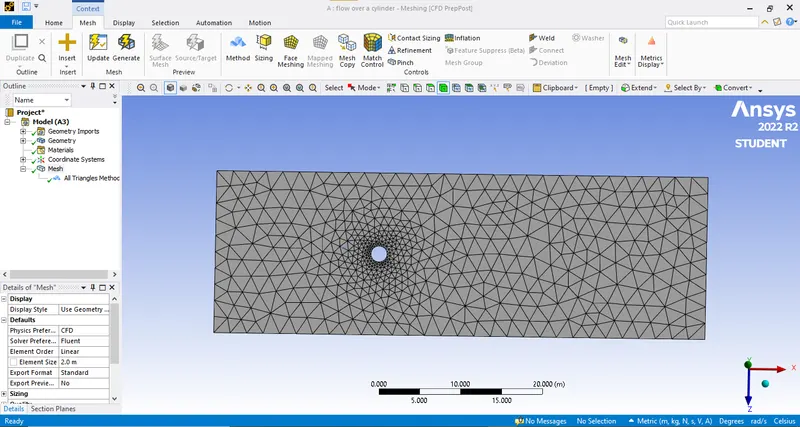
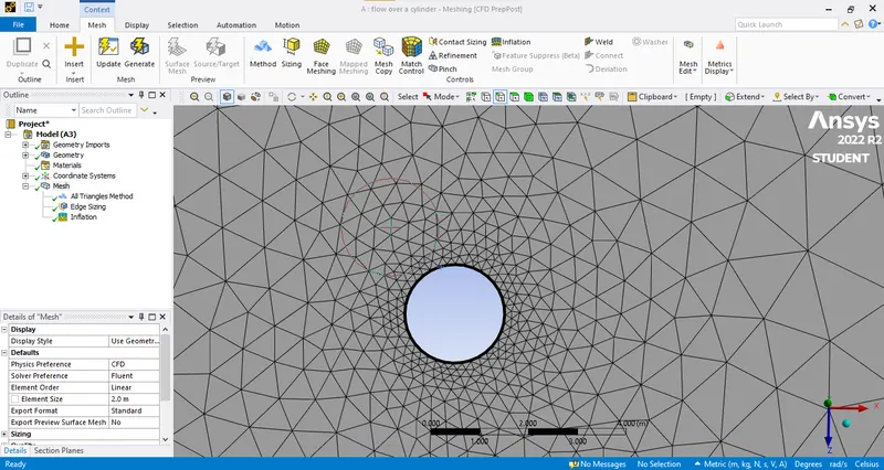
The mesh we had given the element size as 2m.
Before generating the mesh we need to add the Sizing to the wall of the cylinder and along with that Inflation layers are also added to capture the mesh more accurately and precisely.
PART - 1 :- Simulating the flow with the steady and unsteady case and calculate the Strouhal Number for Re= 100.
CASE - A :-Steady flow with Re 100.
SETUP
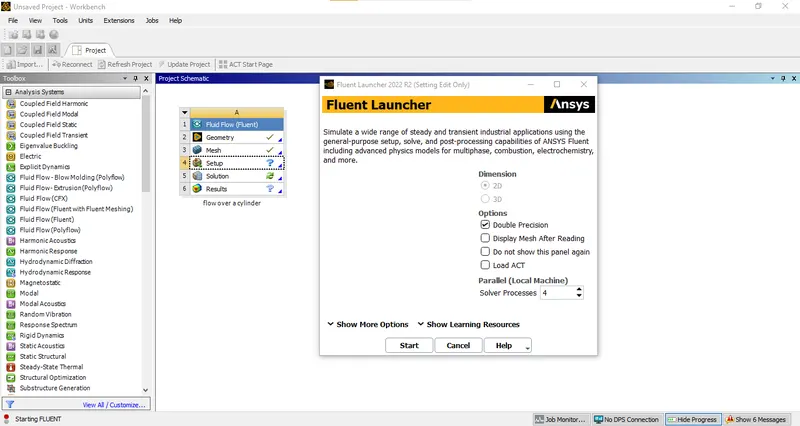
We are simulating the flow with the reynolds number of 100 so we need to calculate the flow velocity required to carried out so from the equation we had ,
Re = ( [ ρ*u*D ] / μ )
We knew Re = 100 , ρ = 1 , D = 2 , μ = 0.05. From the above values we get the Flow velocity as 2.5 (m/s).
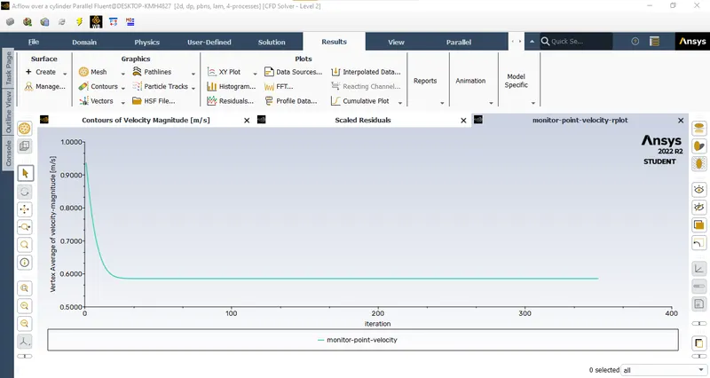
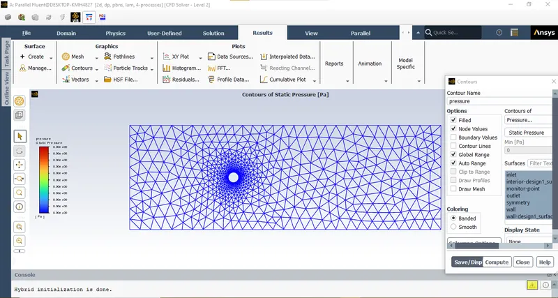
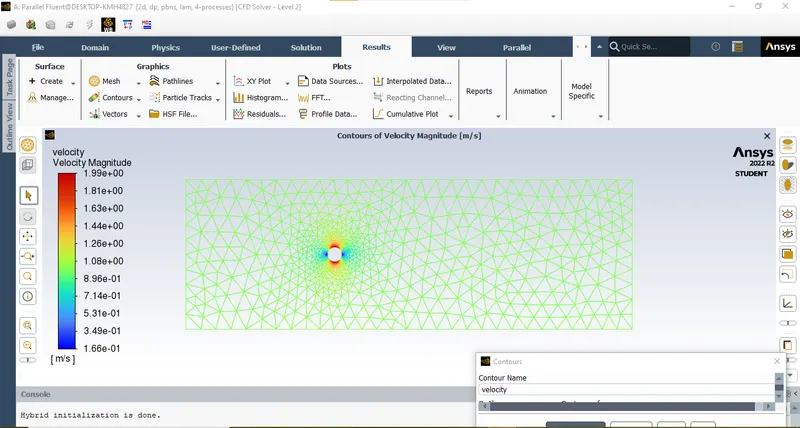
So we run the simulation and capture the velocity, pressure contours along with the for having to identify the vortex shedding we need to first add the monitor point at the particular distance so that it helps in getting the vortex shedding frequencies.
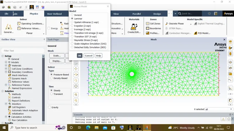
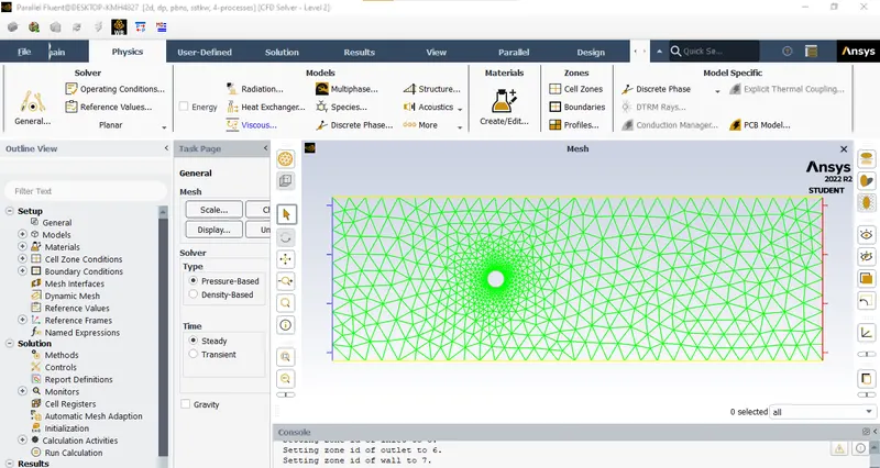
Here we are using the material as User manual because we are adding the values of the density and dynamic viscosity values manually and the flow type as laminar.
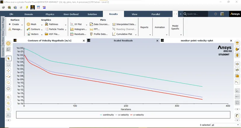
Scaled Residuals
Monitor Point Velocity
Contours for Static Pressure
Contours for Velocity
CASE - B : Unsteady flow with Re = 100.
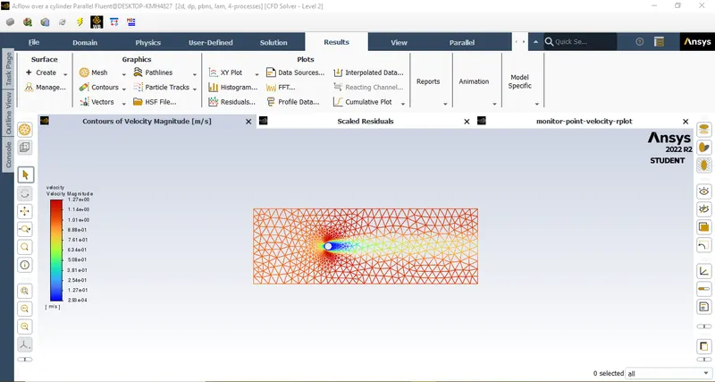
So we run the simulation and capture the velocity, pressure contours along with the Drag Coefficient , Lift Coefficient and for having to identify the vortex shedding we need to first add the monitor point at the particular distance so that it helps in getting the vortex shedding frequencies.
Here we are using the material as User manual because we are adding the values of the density and dynamic viscosity values manually and the flow type as laminar- Transient. Here we are
going to use Turbulent.
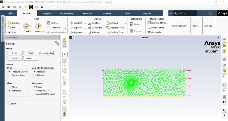
Scaled Residual
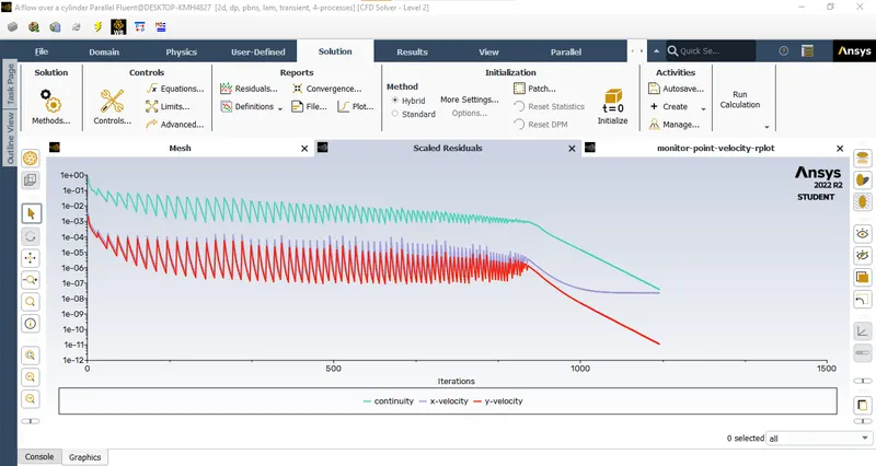
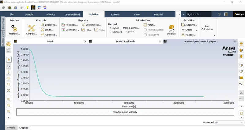
Monitor Point Velocity
Contours for Static Pressure
Contours for Velocity
Strouhal Number calculations:
Strouhal no. is directly proportional on frequency of vertex shedding. In steady state analysis we cannot find out the frequency. So in the steady state case strouhal no. is not calculated.
In the transient case analysis, strouhal no. is calculated from FFT plot.
Sr = ( [0.4 * 2] / 2.5 ) = 0.32
| PART 2:- STEADY FLOW WITH Re - 10,100,1000,10000,100000 |
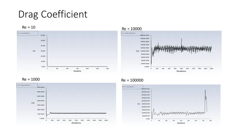
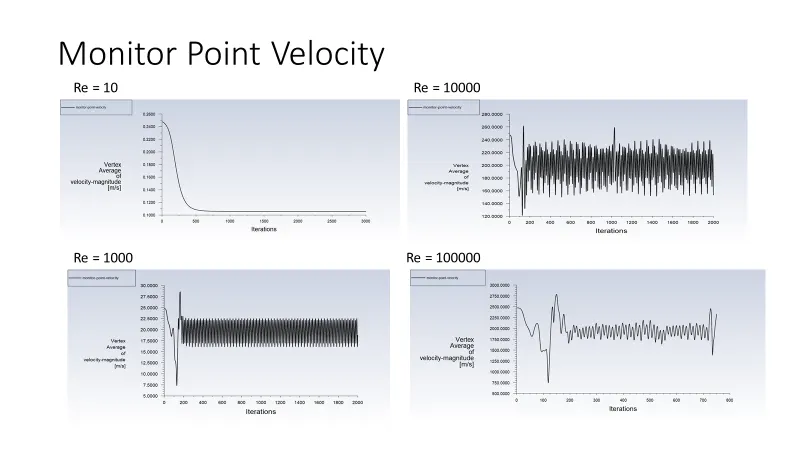
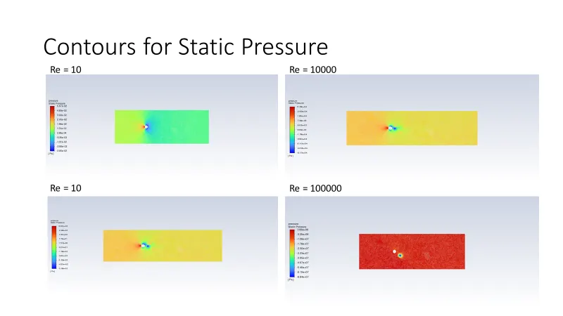
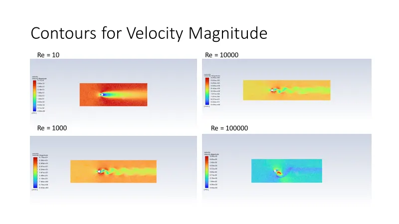
Drag Coefficient :
In fluid dynamics, the drag coefficient is a dimensionless quantity that is used to quantify the Drag or resistance of an object in a fluid environment, such as air or water. It is used in the Drag equation in which a lower drag coefficient indicates the object will have less aerodynamics or hydrodynamics drag. The drag coefficient is always associated with a particular surface area.
The drag coefficient of any object comprises the effects of the two basic contributors to Fluid Dynamic drag: Skin Friction and form drag. The drag coefficient of a lifting airfoil or Hydrofoil also includes the effects of Lift inducted drag. The drag coefficient of a complete structure such as an aircraft also includes the effects of interference drag.
Cd = ( D * 2) / ( ρ * A * V^2 )
Where,
D = Drag Force
ρ = Density
A = Area of Sphere
V = Flow Velocity
Lift Coefficient :-
The lift coefficient (C ) is a dimensionless coefficent that relates the lift generated by a lifting body to the Fluid density around the body, the fluid velocity and an associated reference area. A lifting body is a foil or a complete foil-bearing body such as a fixed wing aircraft. C is a function of the angle of the body to the flow, its Reynolds number and its mach number. The section lift coefficient c refers to the dynamic lift characteristics of a two dimensional foil section, with the reference area replaced by the foil chord.
Cl = ( 2 * L ) / ( ρ * A * V^2 )
Where ,
L = Lift Force
ρ = Density
A = Area of sphere
V = Flow Velocity
Conclusions:
The following conclusions made from the above analysis:
1. Vortex shedding is depends upon the Reynolds number of the viscous flow.
2. Vortex shedding is generated in both steady and unsteady simulations.
3. If we increase the mesh quality, fluid flow behaviour is easily analysed.
4. strouhal no. is calculated in transient simulation because in transient study we can find flow time easily and calculate the frequency of oscillations and find strouhal no.
5.With increase in the Reynolds Number , then Drag Coefficient reduces and Lift Coefficient increases .