Week 2 - Flow over a Cylinder.

Aim:

To Simulate the flow over a cylinder and explain the phenomenon of Karman vortex street.

Objective:

1.To Calculate the coefficient of drag and lift over a cylinder by setting the Reynolds number to 10,100,1000,10000 & 100000. (Run with steady solver)

2.Simulate the flow with the steady and unsteady case and calculate the Strouhal Number for Re= 100.

Introduction:

Vortex shadding:

vortex shedding is an oscillating flow that takes place when a fluid such as air or water flows past a bluff (as opposed to streamlined) body at certain velocities, depending on the size and shape of the body. In this flow, vortices are created at the back of the body and detach periodically from either side of the body forming a Von Karman vortex street. The fluid flow past the object creates alternating low-pressure vortices on the downstream side of the object. The object will tend to move toward the low-pressure zone.

If the bluff structure is not mounted rigidly and the frequency of vortex shedding matches the resonance frequency of the structure, then the structure can begin to resonate, vibrating with harmonic oscillations driven by the energy of the flow. This vibration is the cause for overhead power line wires humming in the wind, and for the fluttering of automobile whip radio antennas at some speeds. Tall chimneys constructed of thin-walled steel tubes can be sufficiently flexible that, in air flow with a speed in the critical range, vortex shedding can drive the chimney into violent oscillations that can damage or destroy the chimney.

Reynolds Number (Re):

Reynolds number for a flow is a measure of the ratio of inertial to viscous forces in the flow of a fluid around a body.

Re = rho*V*d/Dynamic Viscosity

The range of Re values will vary with the size and shape of the body from which the eddies are being shed, as well as with the kinematic viscosity of the fluid. Over a large Re_d range (47<Re_d<10⁵ for circular cylinders; reference length is d: diameter of the circular cylinder) eddies are shed continuously from each side of the circle boundary, forming rows of vortices in its wake. The alternation leads to the core of a vortex in one row being opposite the point midway between two vortex cores in the other row, giving rise to the distinctive pattern shown in the picture. Ultimately, the energy of the vortices is consumed by viscosity as they move further downstream, and the regular pattern disappears.

Strouhal number (St):

Strouhal number is a dimensionless number describing oscillating flow mechanisms.

The Strouhal number is often given as

St = f*d/u

Where,

f is the frequency of vortex shading,

L is the characteristic length and

U is the flow velocity.

Co-efficient of drag:

In fluid dynamics, the drag coefficient(cd) is a dimensionless quantity that is used to quantify the drag or resistance of an object in a fluid environment, such as air or water. It is used in the drag equation in which a lower drag coefficient indicates the object will have a less aerodynamic or hydrodynamic drag. The drag coefficient is always associated with a particular surface area.

The drag coefficient of any object comprises the effects of the two basic contributors to fluid dynamic drag: skin friction and form drag. The drag coefficient of a lifting airfoil or hydrofoil also includes the effects of lift-induced drag. The drag coefficient of a complete structure such as an aircraft also includes the effects of interference drag.

The drag coefficient Cd">CdCd is defined as

Cd=2⋅Fdρu2A">Cd=2⋅Fdρu2ACd=2⋅Fdρu2A

where:

Fd">FdFdis the drag force, which is by definition the force component in the direction of the flow velocity,

ρ">ρρ is the mass density of the fluid,

u">uuis the flow speed of the object relative to the fluid,

A">AA is the reference area.

Co-efficient of Lift:

The lift coefficient (CL">CLCL) is a dimensionless coefficient that relates the lift generated by a lifting body to the fluid density around the body, the fluid velocity, and an associated reference area. A lifting body is a foil or a complete foil-bearing body such as a fixed-wing aircraft. C_L is a function of the angle of the body to the flow, its Reynolds number, and its Mach number. The section lift coefficient c_l refers to the dynamic lift characteristics of a two-dimensional foil section, with the reference area replaced by the foil chord.

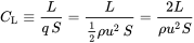
where

is the lift force,

is the relevant surface area and

q is the fluid dynamic pressure, in turn, linked to the fluid density, and to the flow speed.

Procedure:Case-1:

Geometry:

A plate with the dimension of 20*60m is created using spaceclaim.

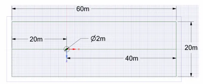
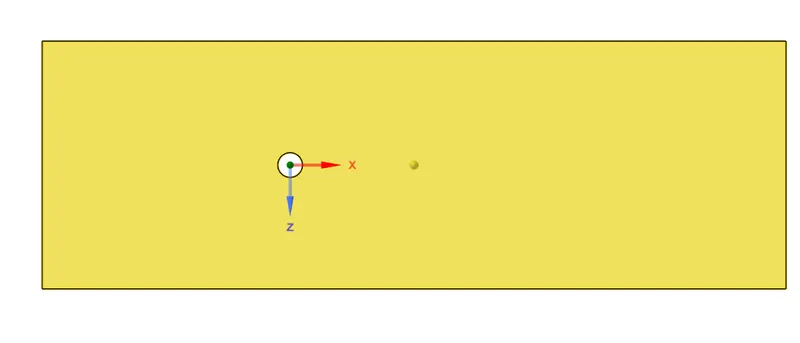
Now,we want to simulate effect of fluid flow over cylinder, select the circle and delete it.

Meshing:-

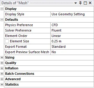
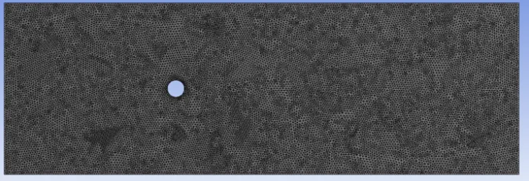
• Now in the mesh mode we set the mesh size, edge sizing and give inflation layers to the cylinder.
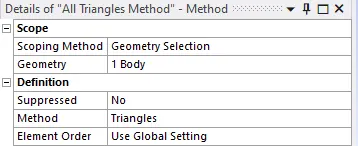
• The mesh size given is 0.25m (Method: Initially, Ansys meshing creates a quadrilateral dominant mesh. We need to convert it into Triangles.

  Go to Mesh→ Insert → Method → Select face → Method(Triangles) →Generate Mesh">Go to Mesh→ Insert → Method → Select face → Method(Triangles) →Generate MeshGo to Mesh→ Insert → Method → Select face → Method(Triangles) →Generate Mesh),

  

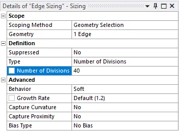
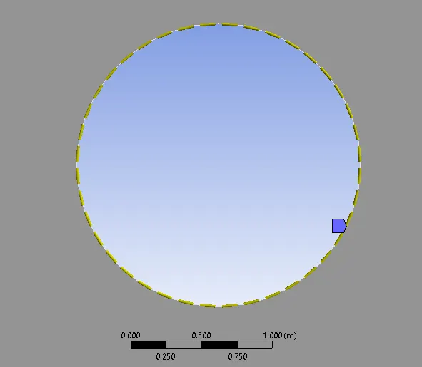
• edge sizing 4 (Sizing: The cylinder we have is not perfectly circular, so if we proceed like that geometry there might be inaccuracy in results. This option will help us to create smooth curves by dividing the circle into large numbers of edges.

  Go to Sizing→ Select Edge→ Type (Number of divisions)→ Enter number and Generate Mesh">Go to Sizing→ Select Edge→ Type (Number of divisions)→ Enter number and Generate MeshGo to Sizing→ Select Edge→ Type (Number of divisions)→ Enter number and Generate Mesh) after edge sizing image is shown below.

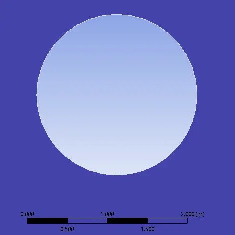
And the obtained mesh is shown below -

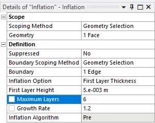
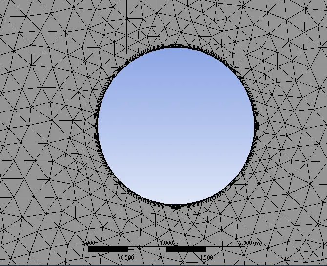
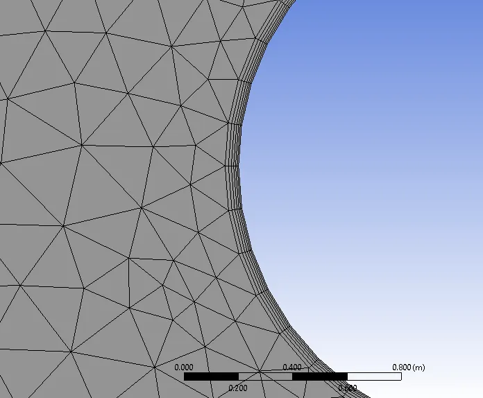
• 6 layers inflation layers with first layer thickness and first layer height of 0.005(Inflation: In order to resolve boundary over the cylinder we will require finner mesh around the cylinder. This option will let us create a finner 'body-fitted mesh' as the flow around the cylinder is quite important.)

Mesh Quality : -

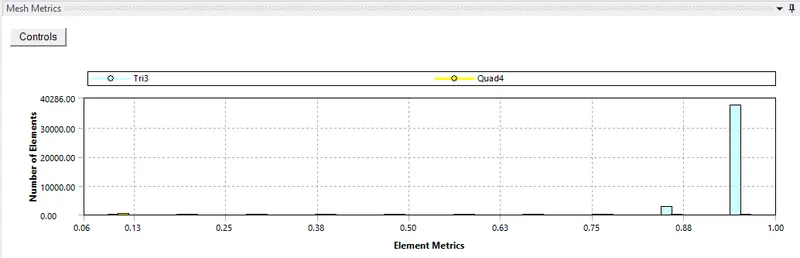
Skewness quality:

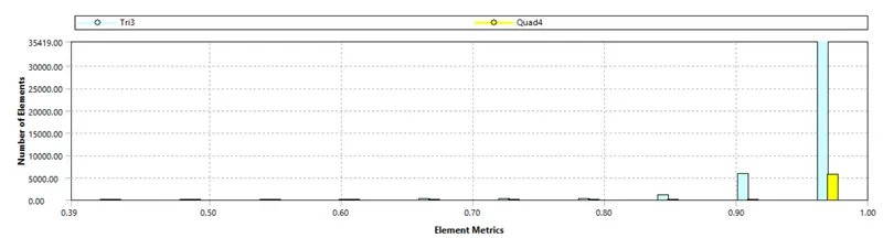
The above graph shows better mesh quality and skewness quality can obtain mesh independent output which can be used for the simulation.

Part Name :-

To set the desired boundaries and to give boundary conditions part naming is to be done after creating the mesh into to the Ansys mesher.

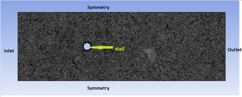
As Shown in above image we can see that as goemetry is symmetric thus symmetry B.C. is used and for cylender no slip wall is used. The naming done according to boundary conditions.

Material Selection: -

The fluid which is used for the simulation is air with constant density and constant dynamic viscosity. To get required Reynolds number only inlet velocity has been changed respectively. The properties of air are given below:

• Density of Fluid: - 1 kg/m^3.
• Dynamic Viscosity: - 0.02 kg/m-s

Solver setting: -

The main important setting for the simulation is reference value setting in the FLUENT. It will change the value with respect to the reference frame from previous value of updated value.

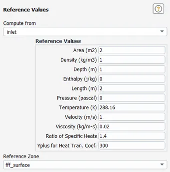
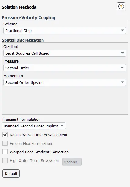
The method which is used for simulation of steady state and unsteady state simulation will be SIMPLE interpolation scheme. Later for the same unsteady state simulation we will be using NITA algorithm to faster the solution time compared to SIMPLE method. It is important to create the report to check for the convergence of simulation.

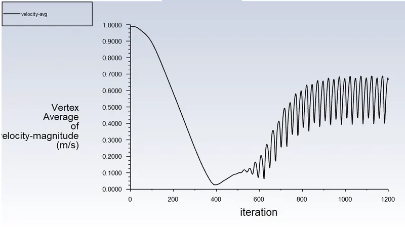
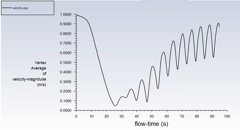
The first report will be vertex average of velocity which will be taking data from 8m from center of cylinder in X-axis. This data will later use to generate strouhal number from this report. Later report which will be required to generate are force report in which coefficient of drag and lift are need to be generated. For coefficient of drag wall should be select as cylinder and there should be 1 in x-axis for drag and respectively 1 for y-axis to calculate lift coefficient.

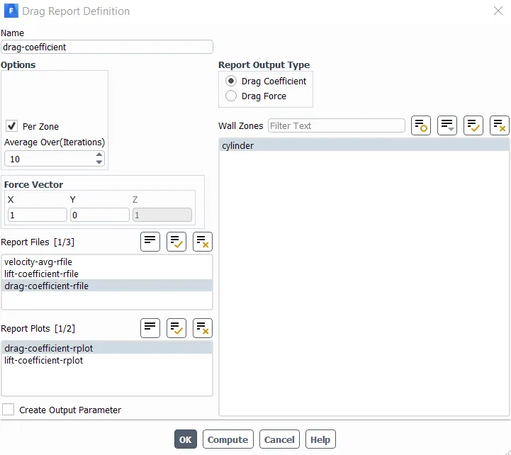
As a steady state solver does not have time as parameter, then to check the animation of flow as it gone past the cylinder, the contour animation plot need to be generated. This can be done after making initialization of solution first, after that solution animation is used as tool to create contour as solution progresses.

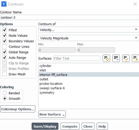
From the above image it can be seen that interior surface need to be selected on which velocity magnitude has to be seen as contour. Similar to it we can also make animation of report of vertex average, residual and coefficient of drag plot.

Result – Steady State Solver for Re = 100

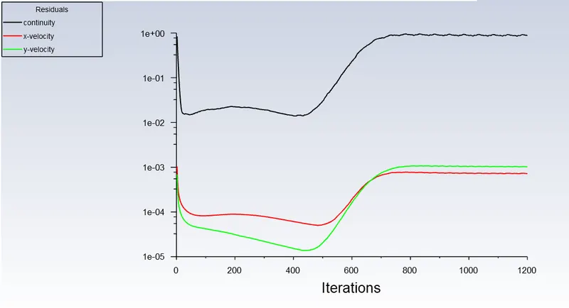
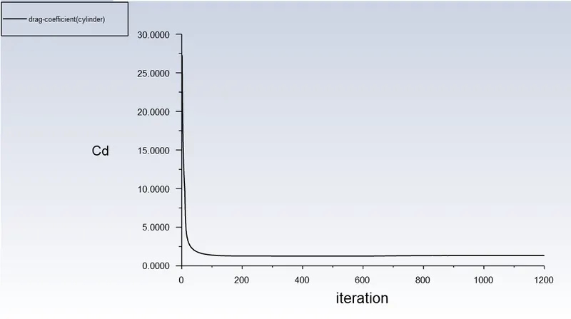
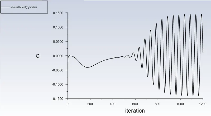
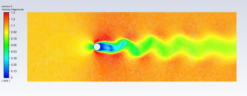
After initialization of solution we run the simulation for 1200 iteration. Here convergence is not mainly important parameter to consider rather than that flow has to be stabilize for longer period so as to capture vortices in the wake region of flow domain.

Residual:

Coefficient of Drag:

Coefficient of Lift:

Vertex average:

Velocity Contour:

Result – Unsteady State Solver with SIMPLE Pressure Velocity Coupling.

Residuals:

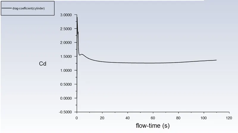
Coefficient of Drag:

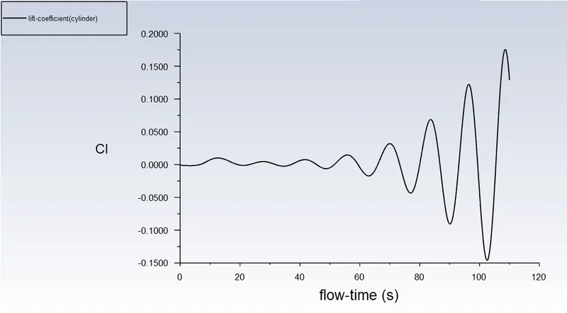
Coefficient of Lift:

Vertex Average:

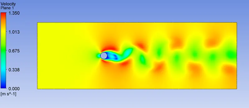
Velocity Contour:

Result – Unsteady State Solver with NITA solver.

The NITA solver as discuss earlier is much faster with respect to simple pressure velocity coupling solver. This solver only accessed by using PISO solver in which further down non-iterative time advancement method is provided. In this method the transient formulation is selected as Bounded second order implicit which is 20% more faster. The setup for NITA is given below

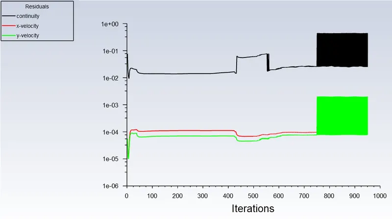
1) Residuals

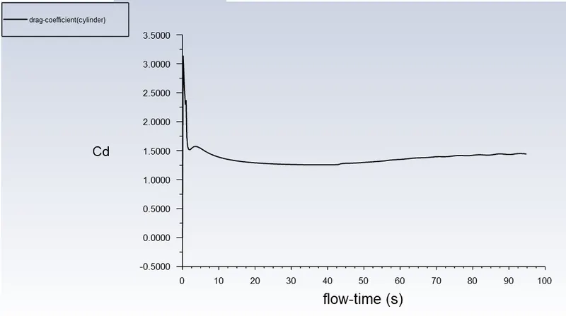
2) Coefficient of Drag

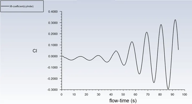
3) Coefficient of Lift

4) Velocity Contour

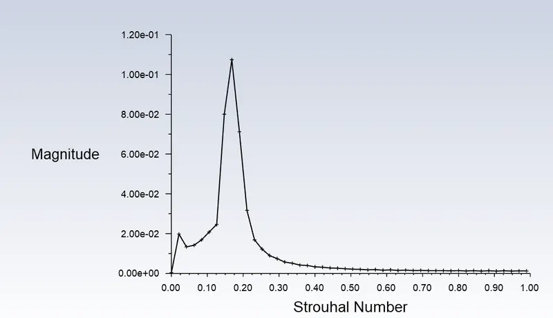
5) Strouhal Number

The strouhal number is calculated by going into plot option in FLUENT in which FFT option has to be choose. In FFT option Y axis function should be Magnitude and X axis function should be strouhal number. After that we need to provide the file of coefficient of lift from simulation and fed to the window to calculate the FFT of lift coefficient which further provide strouhal number. In above case of Unsteady state simulation, the strouhal number is 0.168 which is correct and near to the experimentation result provided by Eric Williams et.al it his paper ‘Simulation of cross flow Induced vibration”

Conclusion: -

• After running both the simulation respectively for steady state and unsteady state simulation it was found that unsteady state simulation provides the result near to the experimentation value validated from the research paper.

Solver	Coefficient of Drag	Coefficient of Lift	Time Taken
Steady State Solver	1.48	0.05	7 min 23 sec
Unsteady State solver (SIMPLE Method)	1.31	0.048	21 min 02 sec
Unsteady state solver (NITA Method)	1.43	0.06	13 min 56 Sec
Experimentation value	1.30	0.045

• If we compare the velocity contour from both steady state simulation and unsteady state simulation, there was more realistic vortex generation is shown in transient simulation as compare to steady state. Hence to capture the flow phenomenon effectively it is better to go with transient solvers.
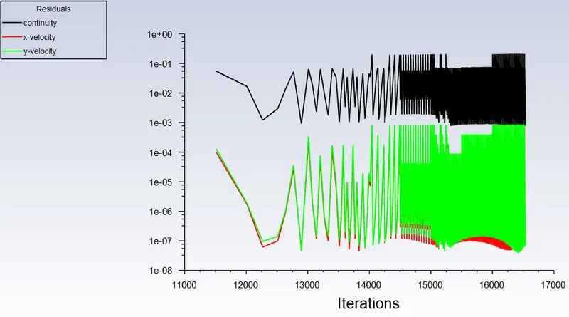
• To make the comment about convergence, it can be seen that from steady state solver the solution gets converged after 600 iterations and after that it shows similar fluctuations. But in case of transient simulation it very hard to predict the convergence from residual, hence we need to take a look at vertex average plot to get the convergence idea.
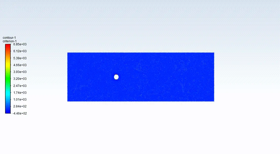
• The q-criterion vortices generation plot was not seen in case of Re = 100 because of, this case still providing vortices in periodic nature in wake region.
• To save the time it was good practice to use Non-Iterative Time Advancement method provided in PISO pressure-velocity coupling method. As it has drastically lower the time of solution compared to SIMPLE pressure-velocity method.

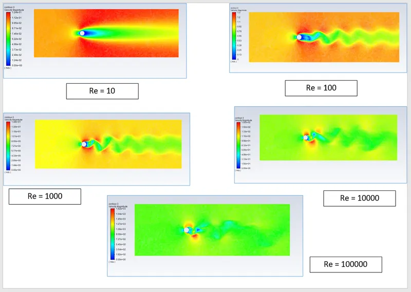
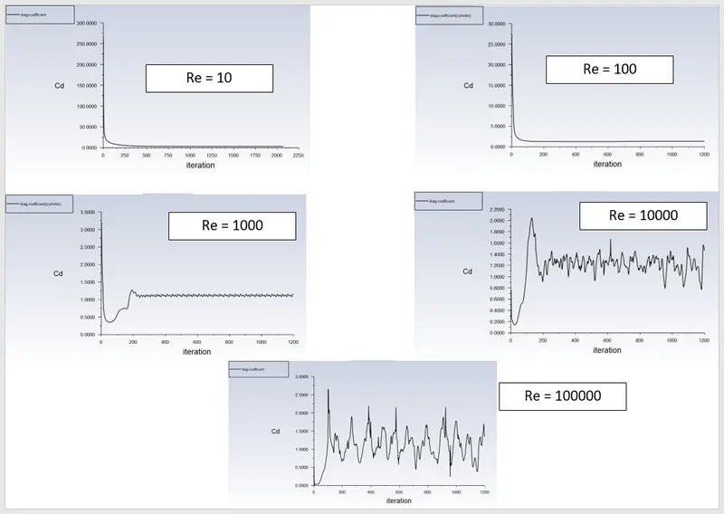
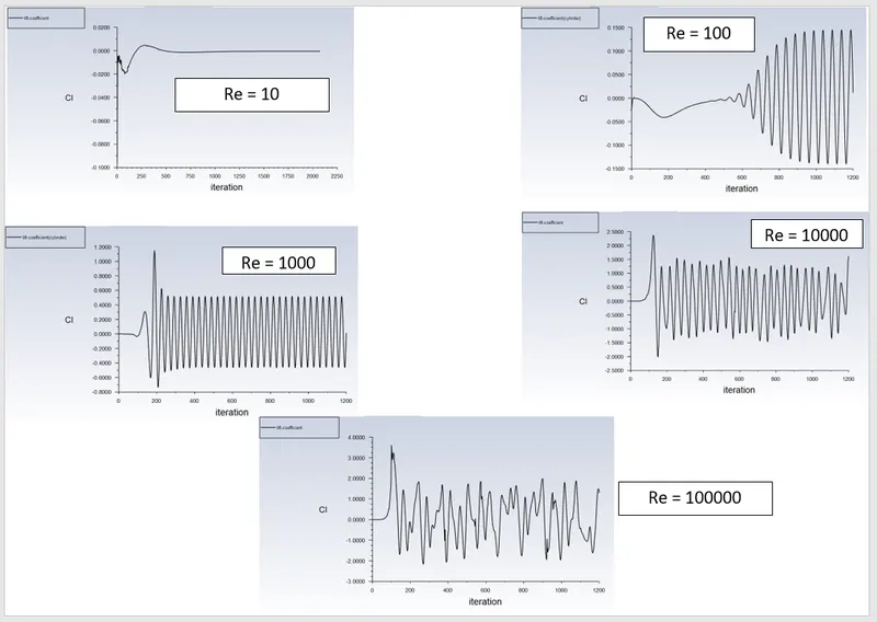
CASE – 2: - Simulation over cylinder with steady solver for Reynold number of 10,1000,10000,100000

1) Velocity Contour plot

2) Coefficient of Drag

3) Coefficient of Lift

4) Animation of velocity Contour for Re = 100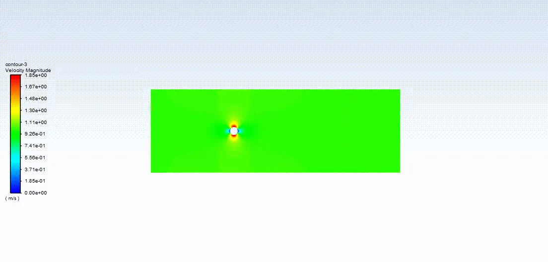

5) Animation of Velocity Contour Re = 1000

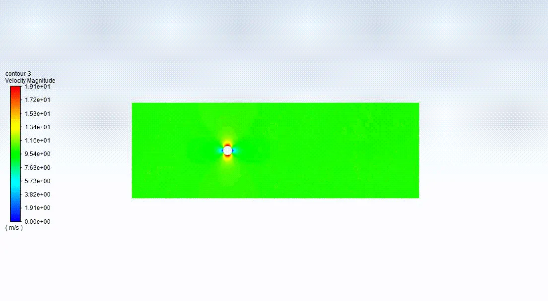
6) Animation of Q criterion

7) Animation of Velocity Contour Re = 10000

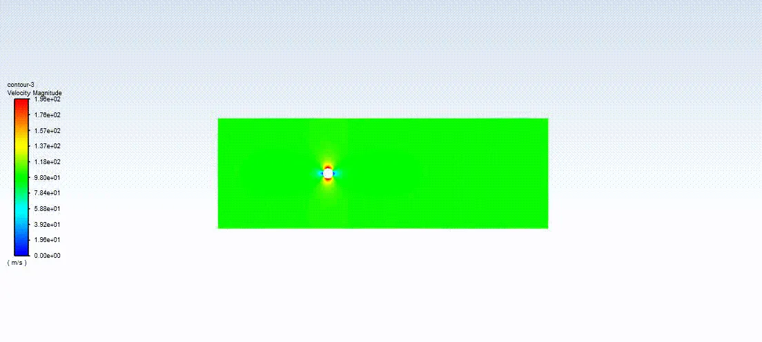
8) Animation of Velocity Contour Re = 100000

Comparison Table of Reynold number with Coefficient of Drag & Lift

Reynolds Number	Coefficient of Drag	Coefficient of Lift
10	3.37	0.0011
100	1.31	0.048
1000	1.08	0.433
10000	1.18	0.562
100000	0.85	0.672

Conclusions:

• In the first case, the flow over a cylinder is simulated for both Steady and unsteady cases with Re=100, and with the results generated the phenomena of Von Karman Vortex Street are also observed.
• Necessary plots are plotted in order to observe that the flow is converged and the vortex shedding is happening.
• Contours are generated in order to observe the flow over a cylinder.
• By plotting Power Spectral Density vs Frequency, the Strouhal number is calculated.

• In the second case,
• six different simulations i.e (Re = 10,100,1000,10000,100000,1000000) are simulated to observe the behavior of the drag and lift coefficients by changing the Reynolds number.
• In order to observe the behavior of the drag coefficients for the simulations, the velocity of the flow is varied to change the Reynolds number and the rest of the parameters are kept constant.
• As we know if the Reynold number is less than 2000, then flow in a pipe is Laminar. Hence we use the Viscous model = Laminar.
• For Re=10, it is observed that there is no formation of vortex shedding and in the rest of the cases, it is clearly observed.
• As per the basic conditions and parameters, the results are validated from the literature.
• As we refine the mesh we need to run more iterations.
• From the above table, it can be concluded that the error percentage is less than 5%.

References:

1. https://www.sciencedirect.com/science/article/pii/S0307904X08000243

2. https://www.thermopedia.com/content/1247/#:~:text=The%20Strouhal%20number%20of%20a,for%20circular%20cylinders%20(tubes).

3. https://www.engineeringtoolbox.com/strouhal-number-d_582.html