Week 2 - Flow over a Cylinder.
Aim:
Simulate the flow over a cylinder and explain the phenomenon of Karman vortex street.
PART-I
Simulate the flow with the steady and unsteady case and calculate the Strouhal Number for Re= 100.
PART-II
- Calculate the coefficient of drag and lift over a cylinder by setting the Reynolds number to 10,100,1000,10000 & 100000. (Run with steady solver)
- Discuss the effect of Reynolds number on the coefficient of drag. [ Results should be validated with any standard literature and error should be within 5 %]
Expected results:
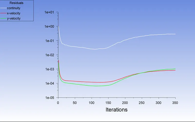
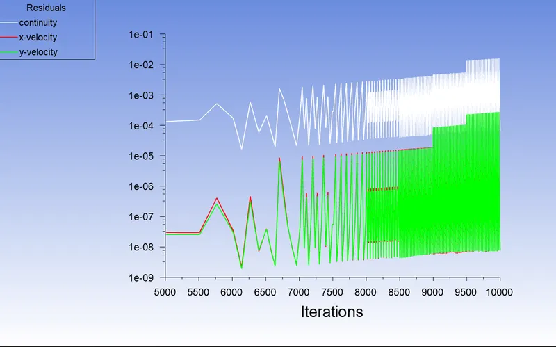
- In both approaches, show that the flow has converged. That is, what quantities or plots need to be looked at to determine that the flow has converged?
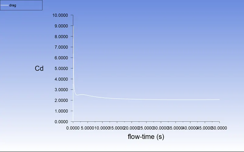
- Plots of the coefficient of drag and lift.
- Plots to show vortex shedding behind the cylinder.
- Mention the referred material (Reference Paper or Fluid Mechanics Textbook) at the end of the challenge submission page.
Procedure:
Phenomenon of Karman vortex street:
- In fluid dynamics, a Karman vortex street is a repeating pattern of swirling vortices, caused by a process known as vortex shedding which is responsible for the unsteady separation of flow of a fluid around blunt bodies.
- It is named after the engineer and fluid dynamicist Theodore von Karman and is responsible for such phenomena as the "singing" of suspended telephone or power lines and the vibration of a car antenna at certain speeds. Mathematical modeling of von Kármán vortex street can be performed using different techniques including but not limited to solving the full Navier-Stokes equations with k-epsilon, SST, k-omega and Reynolds stress, and large eddy simulation (LES) turbulence models, or by numerically solving some dynamic equations such as the Ginzburg-Landau equation.
Reynolds Number: The Reynolds number is a dimensionless number, It is defined as the ratio of inertia force to viscous force.
Formula:
Re=ρ⋅V⋅Dμ
Where, ρ=Density of fluid
V=Velocity of fluid
D= Diameter of cylinder
μ= Dynamic viscosity
Strouhal number: Strouhal number is a dimensionless number describing oscillating flow mechanisms. The frequency at which vortex shedding takes place for an infinite cylinder is related to the Strouhal number by the following equation:
Formula:
St=f⋅DV
Where, St=Strouhal number
f= vortex shedding frequency
D= Diameter of the cylinder
V= Velocity of fluid
Coefficient of Drag (Cd): The coefficient of drag is a dimensionless quantity that is used to determine the drag or resistance of an object in a fluid environment such as air or water.
Formula:
Cd =2⋅Fdρ⋅a⋅v2
Where, Cd= coefficient of drag
Fd=Drag force.
ρ=Density of the fluid
a=Projected area of the object w.r.t which drag force is calculated.
v= Velocity of fluid
Coefficient of lift (Cl): The coefficient of lift is dimensionless quantity that is used to determine the lift of an object in a fluid environment.
Formula:
Cl=2⋅Flρ⋅A⋅V2
Where, Cl=coefficient of lift
Fl=Lift force.
ρ=Density of the fluid
A= Projected area of the object w.r.t which drag force is calculated.
V= Velocity of fluid.
PART-I
Simulate the flow with the steady and unsteady case and calculate the Strouhal Number for Re= 100.
- For steady state simulation Re=100:
Step 1) Creating the geometry: (this is 2D problem)
- The diameter of circle is 2m, and the rectangular surface of 20m width and 60m length the geometry is shown below
Step 2) Meshing:
- In meshing we insert method to change the shape of mesh, In this case we use all triangles method
- The element size is 0.25m
- we are giving the name to boundaries inlet, outlet, symmetry and wall.
Step 3) Set up:
Solver type: Pressure based
Velocity formulation: Absolute
Time: Steady
Viscosity model: laminar
fluent fluid material: User defined
viscosity =0.02 Kg/(m-s), Density=1 kgm3kgm3
Cell zone: fluid type: User defined
Boundaries: inlet (velocity inlet) - Velocity magnitude = 1 m/sec
Outlet (Pressure outlet) - Gauge pressure = 0 pa
Wall: shear condition=No Slip
symmetry = symmetry
Step 4) Result:
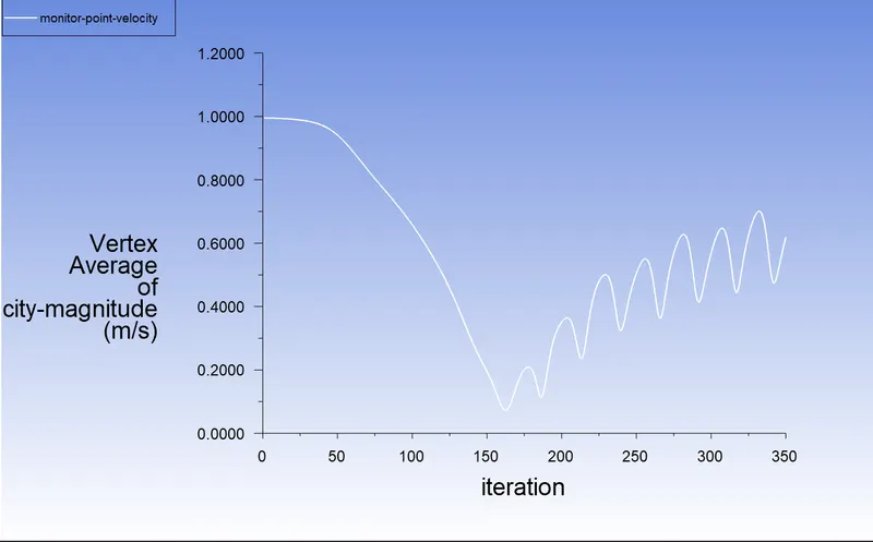
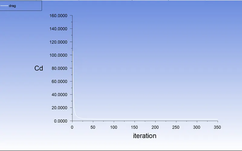
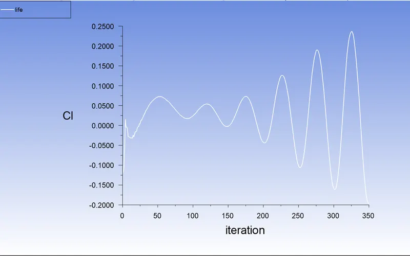
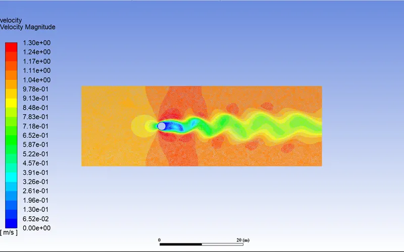
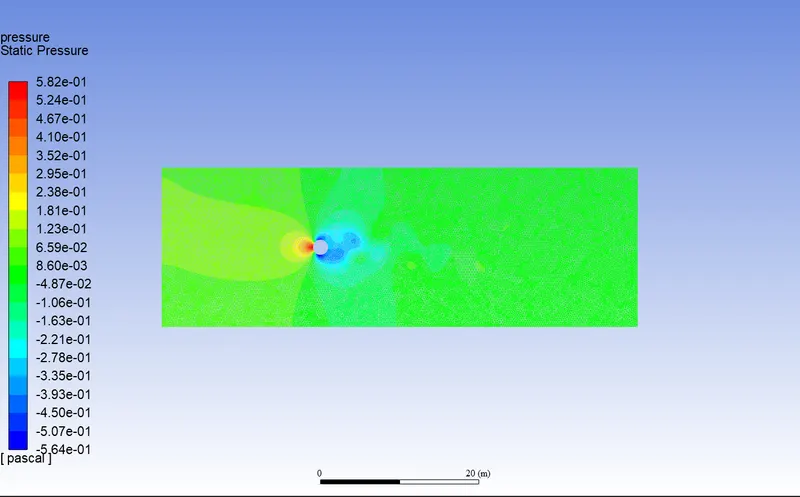
- Solution method used is simple method and we create the report for obtaining the coefficient of drag and coefficient of lift and we create monitor point to right side of the cylinder at distance 10 meter from origin of cylinder for obtaining the vertex average velocity at that point. we create contour plot for velocity and pressure.
Residual plot:
Vertex Average of Velocity Magnitude plot:
Coefficient of Drag plot:
Coefficient of Lift plot:
Velocity contour plot:
Pressure contour plot:
- For unsteady state simulation Re=100:
Set up:
Solver type: Pressure based
Velocity formulation: Absolute
Time: Unsteady
Viscosity model: laminar
fluent fluid material: User defined
viscosity =0.02 Kg/(m-s), Density=1 kg/m3
Cell zone: fluid type: User defined
Boundaries: inlet (velocity inlet) - Velocity magnitude = 1 m/sec
Outlet (Pressure outlet) - Gauge pressure = 0 pa
Wall: shear condition=No Slip
symmetry = symmetry
Residual plot:
Coefficient of Drag plot:
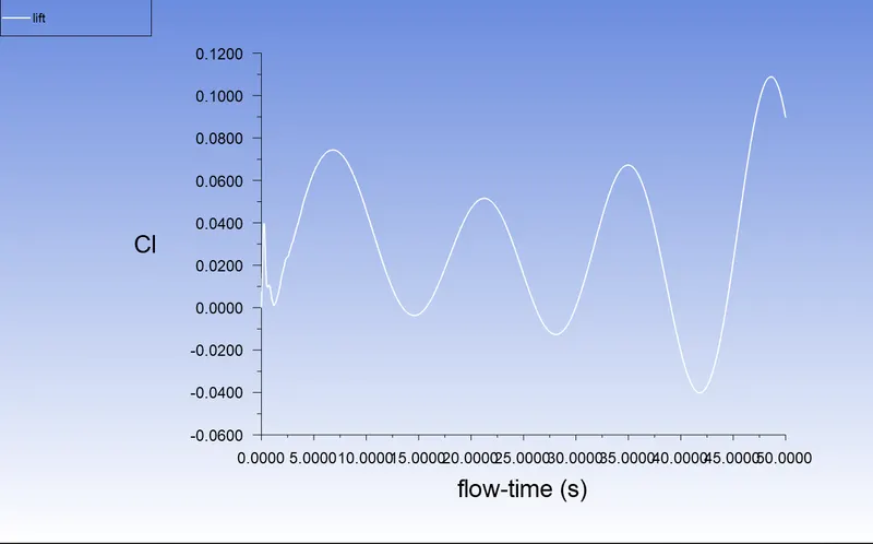
Coefficient of Lift plot:
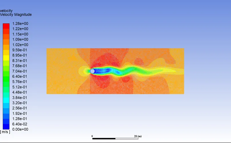
Velocity contour plot:
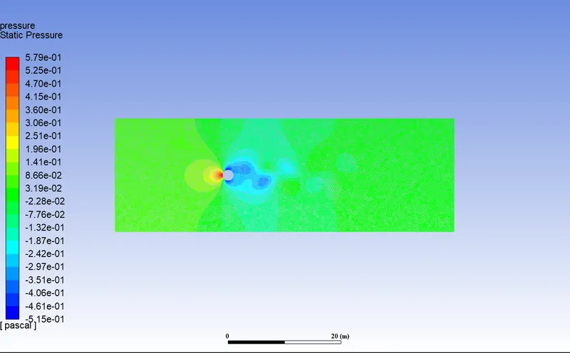
Pressure contour plot:
PART-II
Calculate the coefficient of drag and lift over a cylinder by setting the Reynolds number to 10,100,1000,10000 & 100000. (Run with steady solver)
- For Re=10
Set up:
Solver type: Pressure based
Velocity formulation: Absolute
Time: Steady
Viscosity model: laminar
fluent fluid material: User defined
viscosity =0.02 Kg/(m-s), Density=1 kg/m3
Cell zone: fluid type: User defined
Boundaries: inlet (velocity inlet) - Velocity magnitude = 0.1 m/sec
Outlet (Pressure outlet) - Gauge pressure = 0 pa
Wall: shear condition=No Slip
symmetry = symmetry
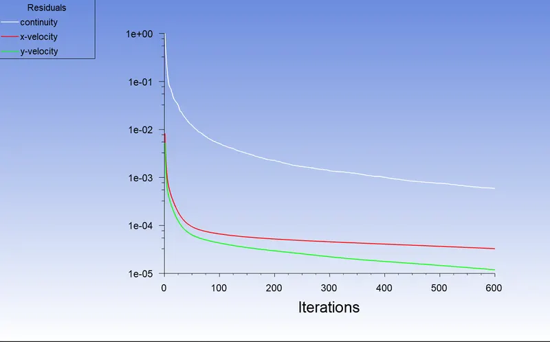
Residual plot:
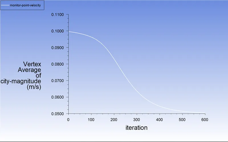
Vertex Average of Velocity Magnitude plot:
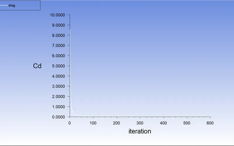
Coefficient of Drag plot:
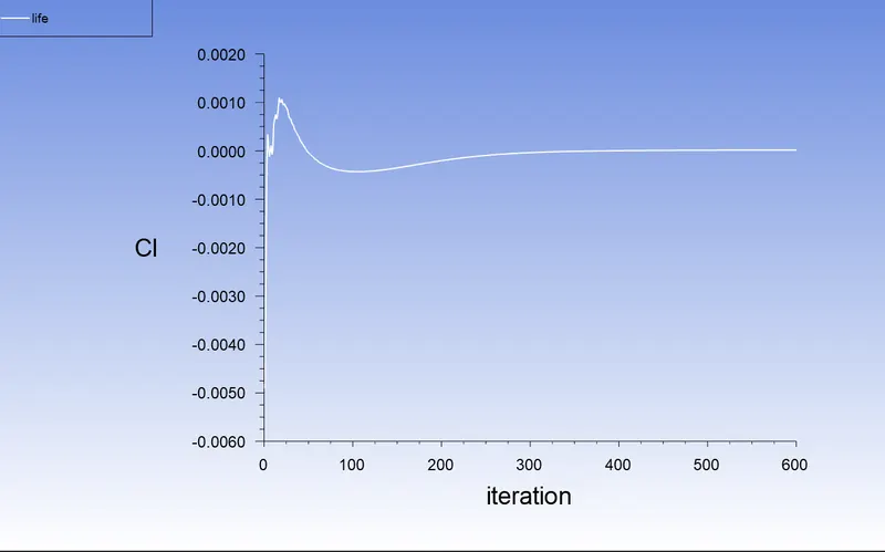
Coefficient of Lift plot:
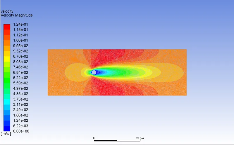
Velocity contour plot:
Pressure contour plot:
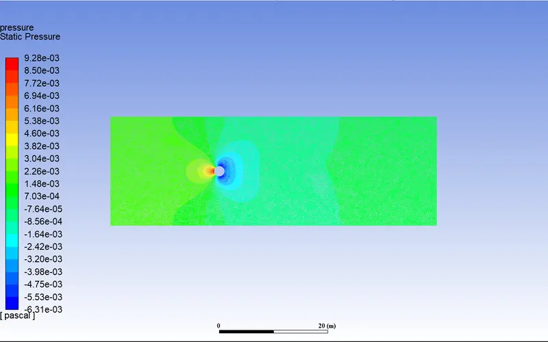
- For Re=100 we have already calculate the coefficient of drag and lift value in part 1
- For Re=1000
Set up:
Solver type: Pressure based
Velocity formulation: Absolute
Time: Steady
Viscosity model: laminar
fluent fluid material: User defined
viscosity =0.02 Kg/(m-s), Density=1 kg/m3
Cell zone: fluid type: User defined
Boundaries: inlet (velocity inlet) - Velocity magnitude = 10 m/sec
Outlet (Pressure outlet) - Gauge pressure = 0 pa
Wall: shear condition=No Slip
symmetry = symmetry
Residual plot:
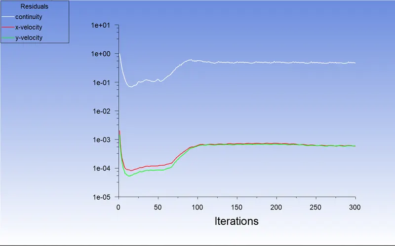
Vertex Average of Velocity Magnitude plot:
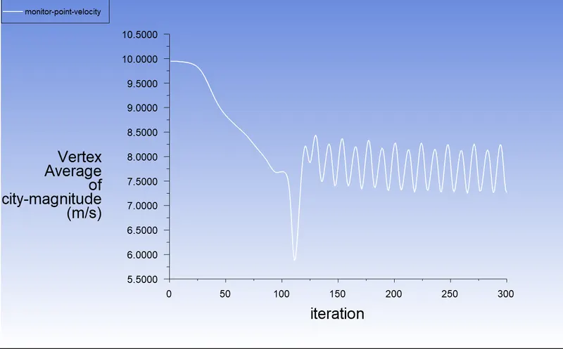
Coefficient of Drag plot:
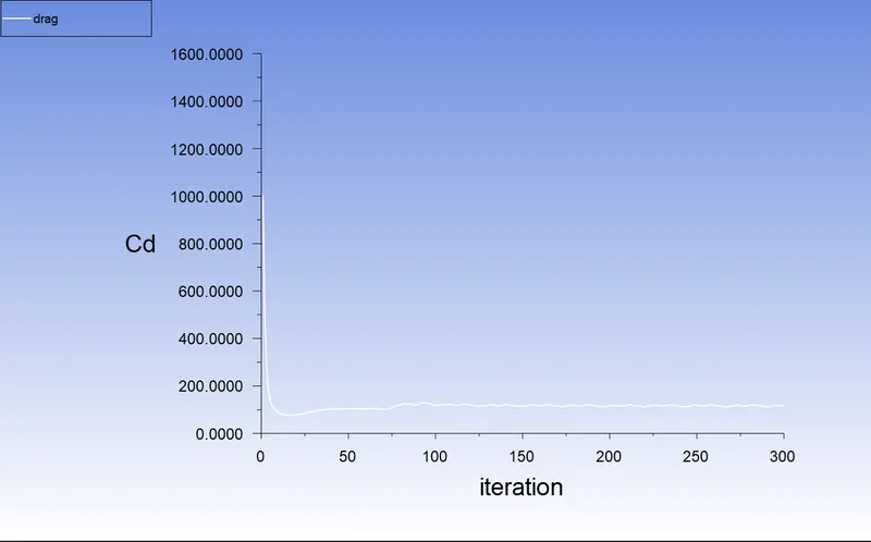
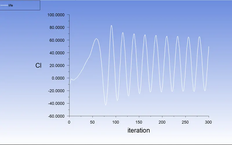
Coefficient of Lift plot:
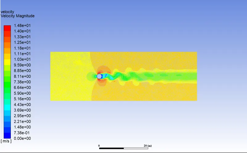
Velocity contour plot:
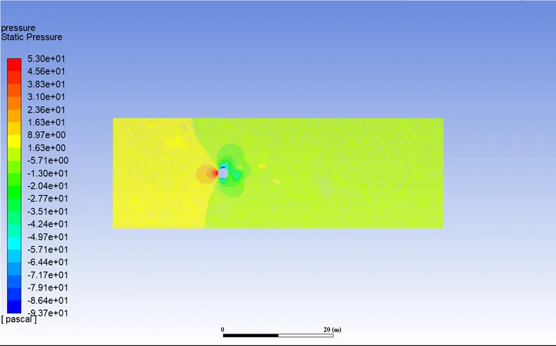
Pressure contour plot:
- For Re=10000
Set up:
Solver type: Pressure based
Velocity formulation: Absolute
Time: Steady
Viscosity model: laminar
fluent fluid material: User defined
viscosity =0.02 Kg/(m-s), Density=1 kg/m3
Cell zone: fluid type: User defined
Boundaries: inlet (velocity inlet) - Velocity magnitude = 100 m/sec
Outlet (Pressure outlet) - Gauge pressure = 0 pa
Wall: shear condition=No Slip
symmetry = symmetry
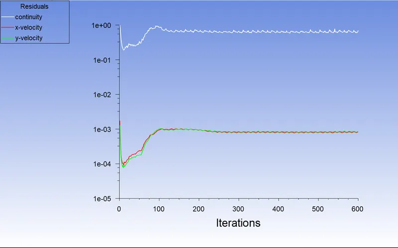
Residual plot:
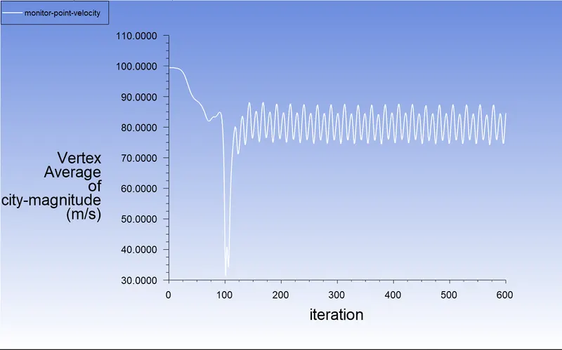
Vertex Average of Velocity Magnitude plot:
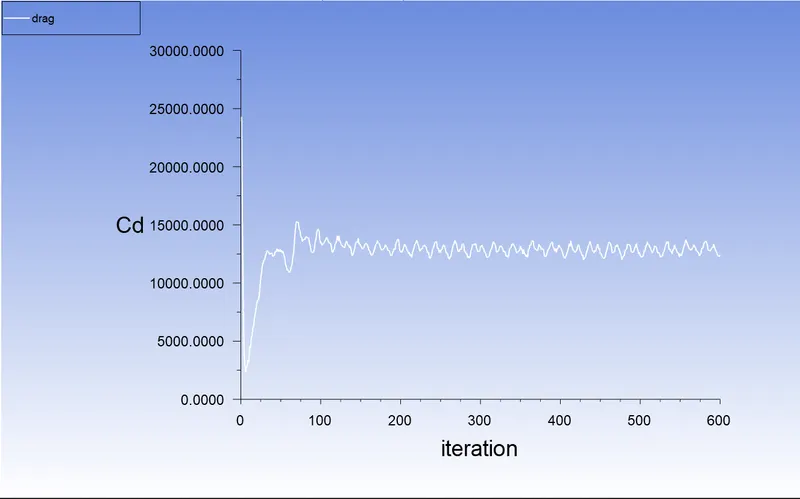
Coefficient of Drag plot:
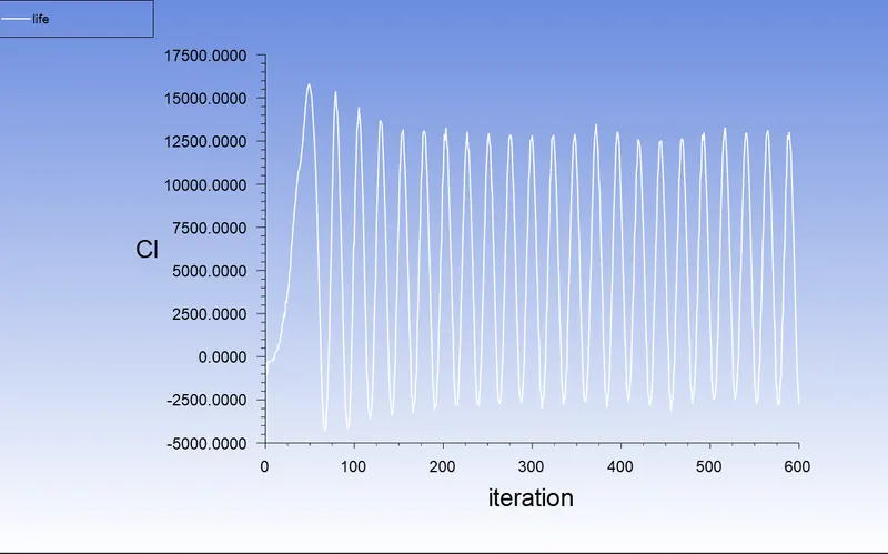
Coefficient of Lift plot:
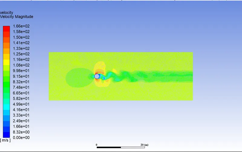
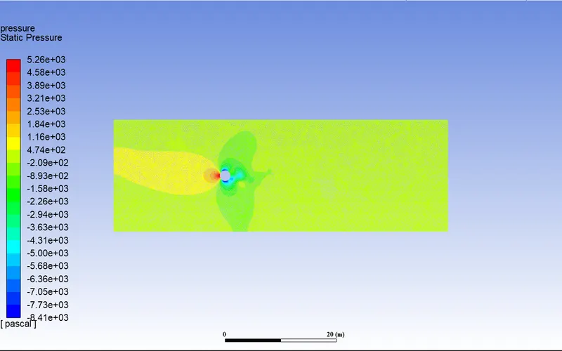
Velocity contour plot:
Pressure contour plot:
- For Re=100000
Set up:
Solver type: Pressure based
Velocity formulation: Absolute
Time: Steady
Viscosity model: laminar
fluent fluid material: User defined
viscosity =0.02 Kg/(m-s), Density=1 kg/m3
Cell zone: fluid type: User defined
Boundaries: inlet (velocity inlet) - Velocity magnitude = 1000 m/sec
Outlet (Pressure outlet) - Gauge pressure = 0 pa
Wall: shear condition=No Slip
symmetry = symmetry
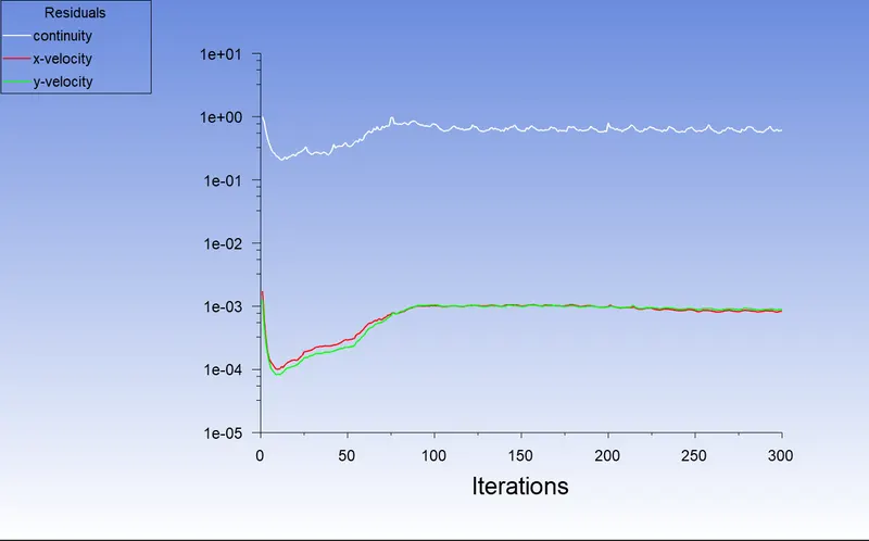
Residual plot:
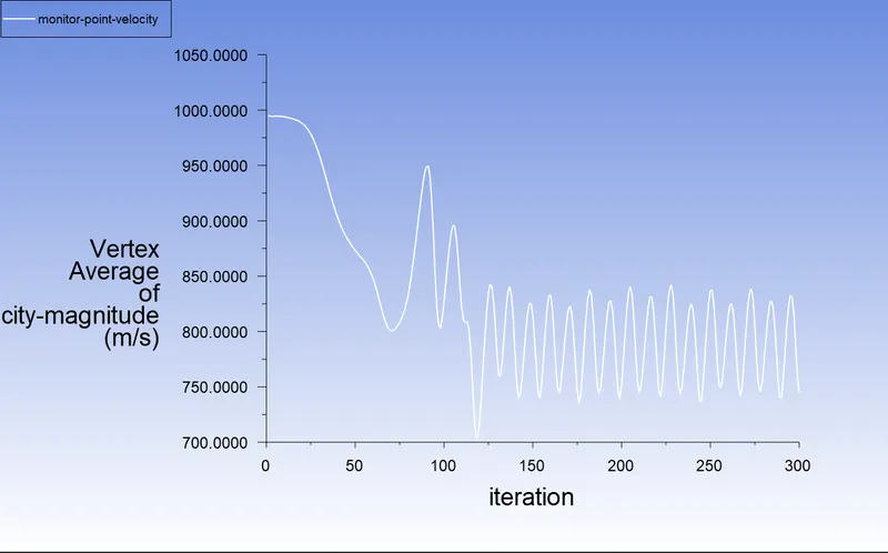
Vertex Average of Velocity Magnitude plot:
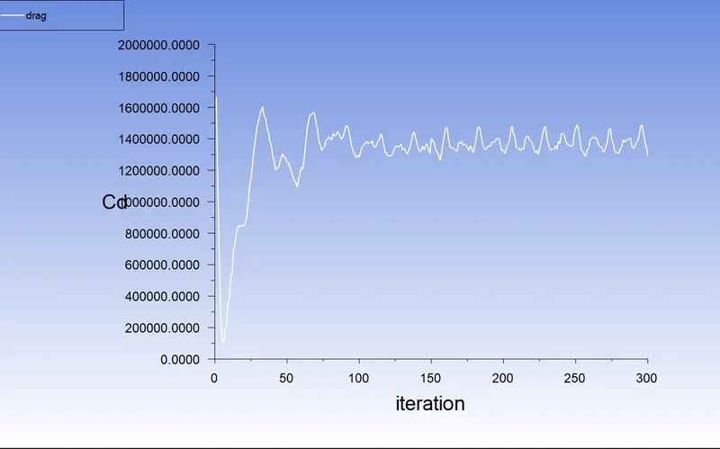
Coefficient of Drag plot:
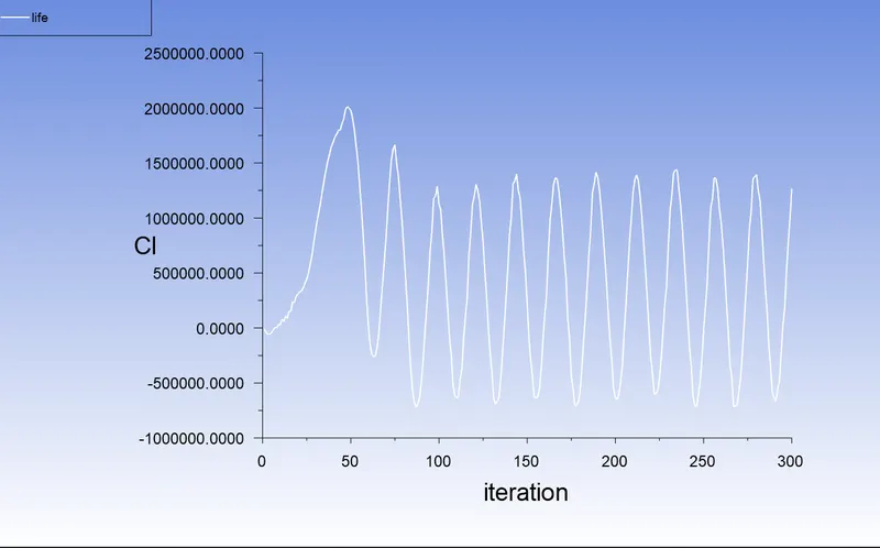
Coefficient of Lift plot:
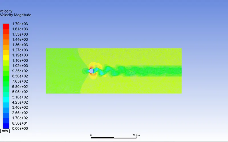
Velocity contour plot:
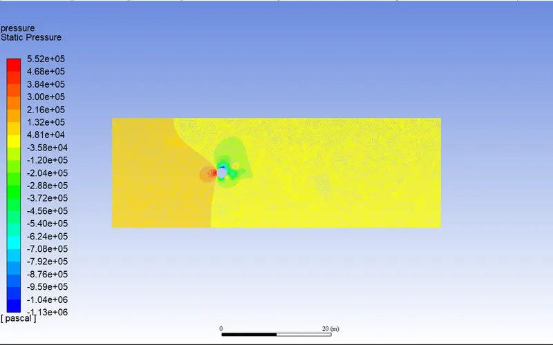
Pressure contour plot:
For the steady state simulation Value of Reynolds no., Coefficient of drag, Coefficient of lift are tabulated as follows:
|
Sr No |
Reynolds No (Re) |
Coefficient of Drag (Cd) |
Coefficient of lift (Cl) |
|
1 |
10 |
3.332 |
-0.0026 |
|
2 |
100 |
1.3147 |
0.1106 |
|
3 |
1000 |
1.1073 |
0.5665 |
|
4 |
10000 |
1.1824 |
0.6629 |
|
5 |
100000 |
0.9585 |
0.6123 |
Conclusion:
- From the above table we can say that the Reynolds number increases then the coefficient of drag is decreases and coefficient of lift is increases.
- The Reynolds number increases in value then the wake region behind the cylinder is also increases.
- The vortex shedding is takes place when Reynolds number is 100 and above value.