Week 2 - Flow over a Cylinder.

Project: Simulate the flow over the cylinder and the demonstration of the Von Karman Vortex.

Abstract:

Simulate the flow over the cylinder. Discuss the effects of Inflation addition layers and Effects of Reynolds number on the Coefficient of the Drag.

------------------------------------------

Part-1: We will discuss steady and Transient Simulation and calculate the Strouhal Number for Reynolds Number=100.

Part-2: Calculate the Drag and lift calculation over the cylinder for the series of the Reynolds Number and show the effect of the Reynolds Number on the Coefficient of the drag.

Part-1:

The study Contains a steady and Unsteady part of the simulation over the cylinder. The Preprocessing of both simulations is the same till the Meshing steps. The following steps are involved in the Preprocessing.

Modeling:

The Simulation uses the 2D-Geometry of the cylinder to calculate the Von Karman Vortex. The Modelling involves the following data

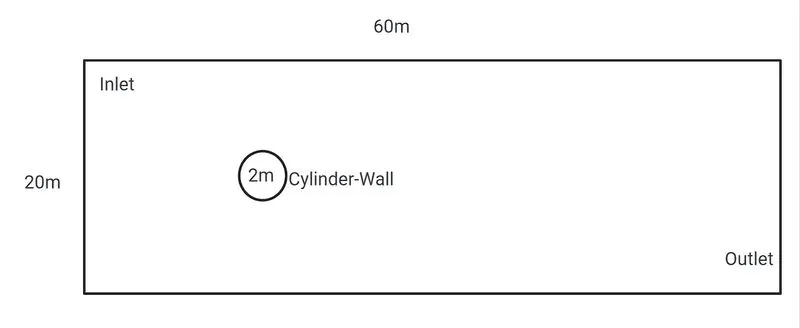
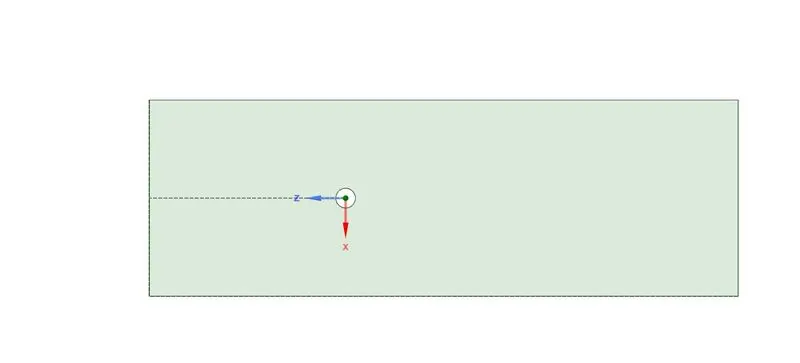
Rough sketch of the geometry. Modeling is done in the Ansys modeling software SpaceClaim. After the modeling step, the meshing is done in the Ansys Mechanical. The following figure gives the modeled geometry of the cylinder. Flow enclose has a dimension of 60 meters. Dimension of the enclose based on the cylinder dimension, Length between the center to the inlet is 10D. The Center to the outlet dimension is 20D. The diameter of the cylinder in my case is 2 meters. The Modelling parameter is calculated based on the Diameter of the Cylinder.

Meshing:

For solving the Navier strokes and energy conversion equation coupled with the continuity equation. This introduces the numerical diffusion and this is approximating the diffusion terms via the central-difference approximation. for this domain is divided for solving the problem.

The iterative meshing is used to find the optimal Meshing. The Iteration of the Domain is done based on the Element size of the Mesh. Before the Iteration, the initial steps involve creating the Triangular Mesh to get more nodes and elements to approximate the accurate solution. The Edge meshing is done to get more division so the finer curve is solved. The Inflation is added to get the more accurate results near the curvature. By keeping the courant number in mind, the dimensionless number distance that any information travels during the time step length within the mesh must be lower than the distance between mesh elements. Numerical Diffusion is the cause of the error in the numerical solution, it can be reduced by using the correct courant number for the simulation. For this Simulation, the Courant number is maintained at less than 1.

Triangular Mesh Domain:

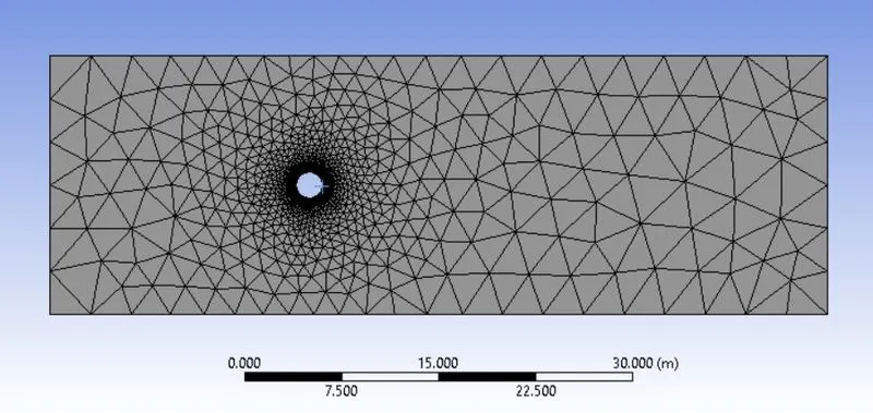
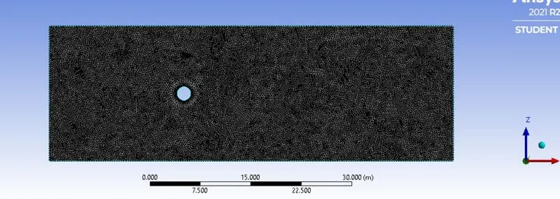
The triangular Mesh domain is used to capture the flow of the region more efficiently. In the Triangular Mesh Nodes and Elements are more than the Quand domain. The Element Size is set to 0.25 m. Updated Mesh looks as Follows

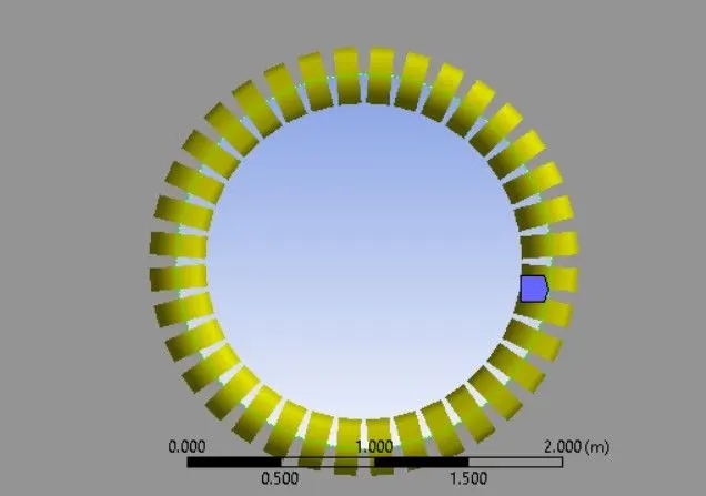
Edge Sizing:

It is done to get the More curvature structure for the cylinder wall. It is divided into 36 Divisions.

Inflation Layers:

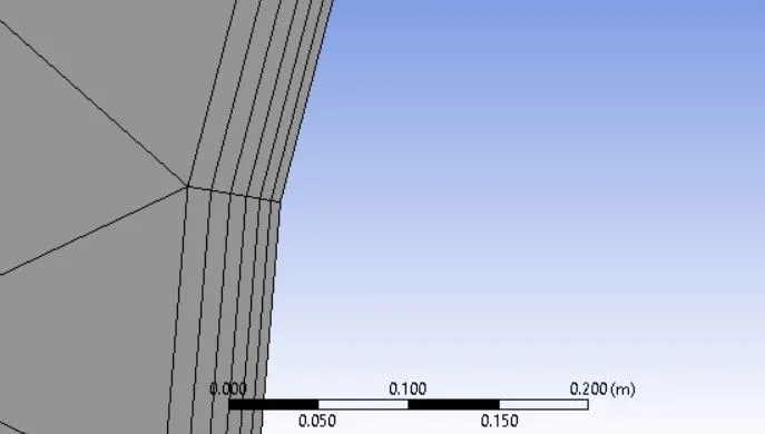
In general, it helps to create the body fitted mesh, Considering the Grid Refinement Factor, Calculating the First Layer Thickness for Laminar Flow = 5e-3 m. On Referring following image First Layer Thickness is Calculated. The growth rate is given as 1.2.

Boundary Condition:

Inlet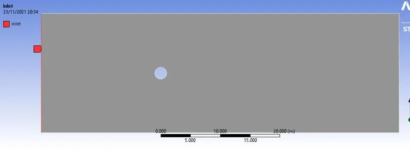
Outlet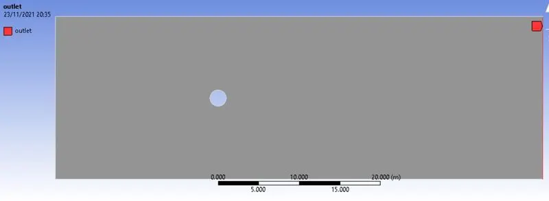
Symmetry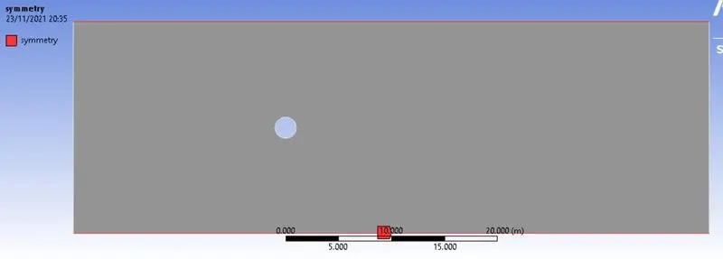
Cylinder Wall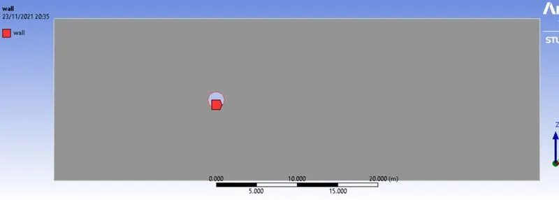

SETUP THE PHYSICS FOR SIMULATION:

The calculation for the Reynolds Number:

A dimensionless number used in fluid mechanics to indicate whether fluid flow past a body is steady or turbulent(Unsteady Flow)

`Re = (rhouL)/ mu`

where Re is the Reynolds number

`rho` is the Density of the fluid = `0.02 (kg)/(m^3)`

`u`is the inlet Velocity of the fluid

`L` is the Length of the Domain = `2 m`

For the above Problem, the Reynolds Number is given as `Re = 100` Calculating the Inlet velocity using the Reynolds Number

`u = (mu*Re)/(rho.L)`

`u = (0.02*100)/(1*2)`

`u=1 m/s`

Using the above formula for series of the Reynolds Number

`Re = 10`	`u=0.1 m/s`
`Re=100`	`u=1 m/s`
`Re=1000`	`u=10 m/s`
`Re=10000`	`u=100 m/s`
`Re=100000`	`u=1000 m/s`

FOR STEADY-STATE SIMULATION:

• Launch the Setup and check for the Boundary Condition Update.

Method:

Type	Pressure-Based
Velocity Formulation	Absolute
Time	Steady State
2D Space	Planar

Material Assigning:

• Create the new material by copying the air and setting the `rho=1 (kg)/(m^3)`(Density) and Viscosity = `0.02 (kg)/(m.s)`
• Open the cell boundary Zone and define the user-defined Fluid region.
• Delete the Properties of the air in the material Assigning tab.
• Make sure the Material Assign as User Material is Defined.

Boundary Condition:

• Inlet: Give the Calculated value for the Inlet Velocity.
• Outlet: Check the Guage Pressure equal to Zero and Check for the Pressure Outlet.
• Cylinder Wall: Check for the No-slip boundary condition for the Wall
• Symmetry: Check for the Symmetry Wall.

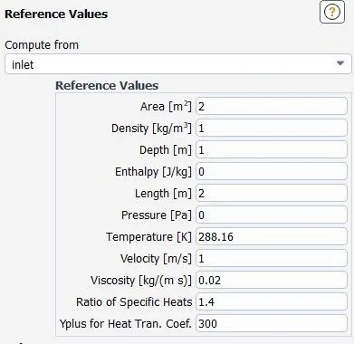
Reference Values:

• Check the Reference Values, Compute using the inlet Condition.
• Check for the Velocity, Viscocity, Area, Length.

Solution:

• Check the Method for Simple in the Solver Section.
• Add the Monitor Point in the Domain using Surface Option in the Post-Processing at a distance of 8m from the Origin. (i.e, From the center of the circle).
• Next Step, Uncheck all the Residuals Plot like Continuity, X- Velocity, and Y- Velocity in the Residual Plot.
• Add the Vertex Average Velocity for the Monitor Point we have created before.
• Add the Coefficient of Lift and Drag by using the Force Report.
• Now initialize the domain using the Hybrid Initialization.
• Create the Velocity and Pressure Contour using the Contour option in the Post Processing.
• Run for 1000 iterations for the Steady State Simulation.

Strouhal Number:

The Strouhal number is a dimensionless number describing oscillating flow mechanisms

`St = (f.D)/u`

For Unsteady Simulation:

Method: Type- PRESSURE BASED and Time = Transient

• Following the Steady Step Process till the Initialization.

Time Step Calculation for the Transient:

`L=60 m and V=1 m/s`

For Calculate Time Step Size we need the frequency of the vortex Shredding.

`f=(St.u)/(D)`-------------------(Equn1)

Where St is the Strouhal number

u is the Inlet Velocity.

D is the Diameter of the cylinder.

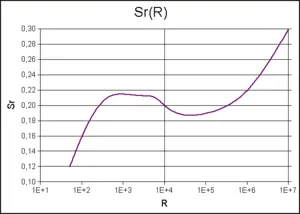
From the Above image, Sr for the Reynolds Number 100 equals 0.164.

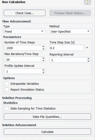
Time Step Size `Deltat=(T)/25` is calculated equals to 0.1964 secs.

Time Step = 306 Iterations.

In this simulation, the Timestep size and Time Step should be greater than or equal to 0.1964 secs and 306 Iterations. I have set the Time Step size 0.2 and Time Step as 1000.

`

PART-1

Results for steady Re=100.

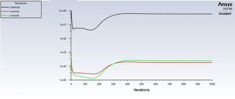
Residual Plot:

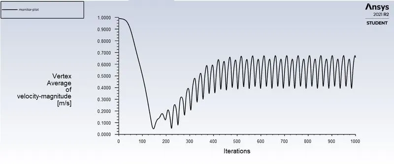
Vertex Average at the Monitor Point:

Velocity Contour

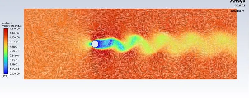
Velocity Contour:

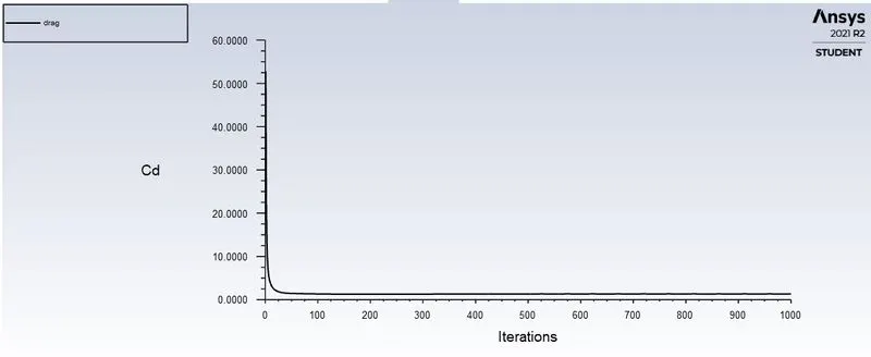
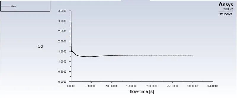
Coefficient of Drag:

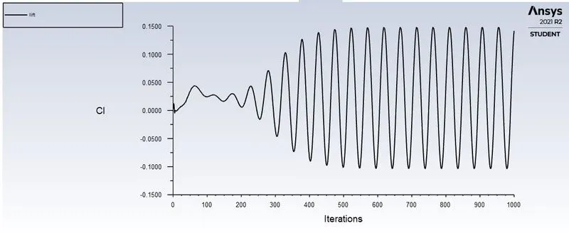
Coefficient of lift:

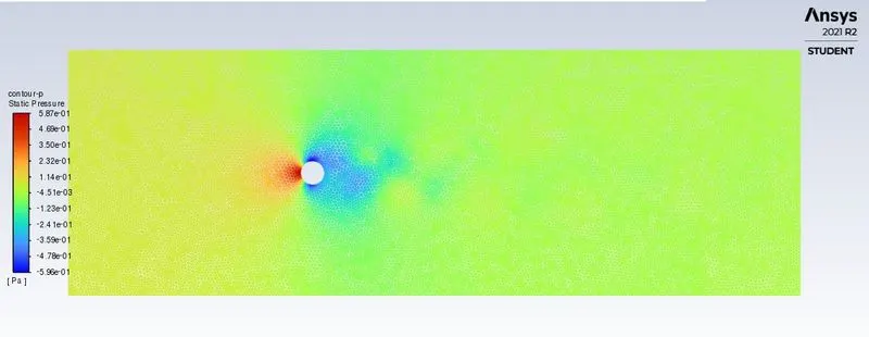
Contour Pressure:

For Unsteady Simulation Reynolds Number-100:

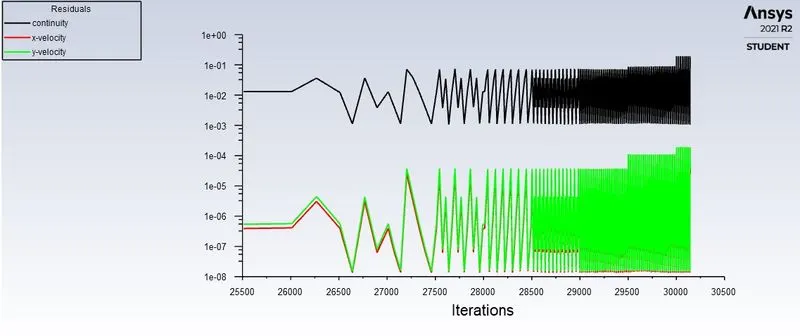
Residual plot:

The time step is set to 0.2 to capture the vortex formed by the cylinder

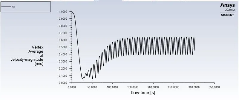
Vertex Average of Velocity plot:

Velocity contour:

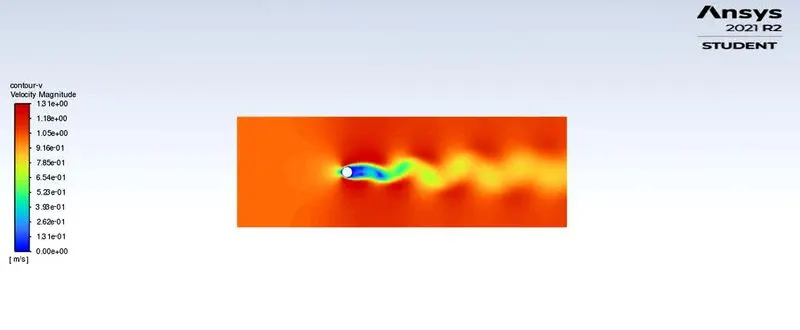
Video plot for the Velocity Contour:

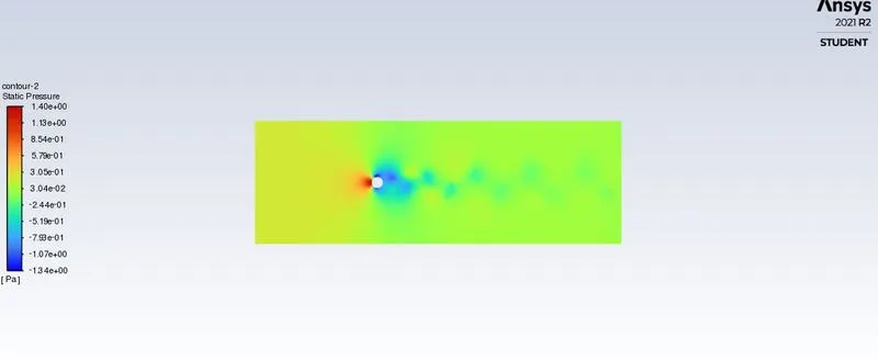
Pressure Contour:

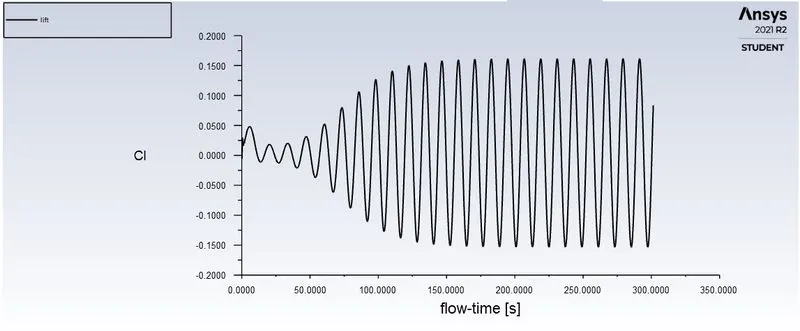
Coefficient of lift:

Coefficient of Drag:

Cd

wall 1.368641

Strohaul Frequency plot:

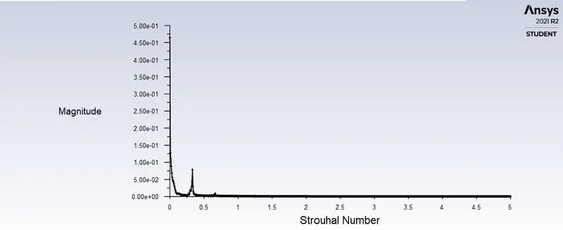
Strouhal Number:

The Plot Vertex Average Velocity shows the frequency of the vortex Shedding is given by

Fluids oscillate 9 times between 250 and 300. So the Frequency is 0.18.

Calculating the Strouhal Number

`Sr =(f*L)/u=(0.18*2)/1`

`Sr=0.36`

PART 2

SERIES OF REYNOLDS NUMBER

REYNOLDS NUMBER =10

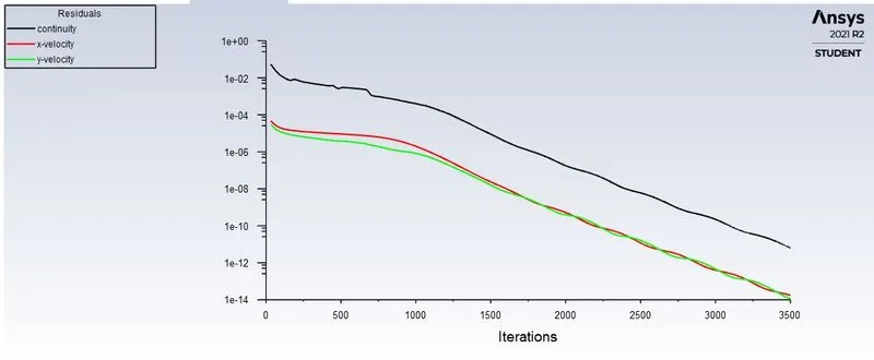
RESIDUAL PLOT:

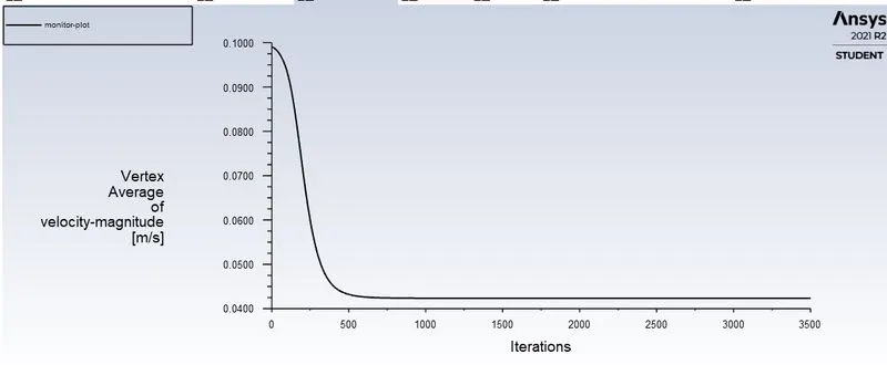
Vertex Average of Velocity plot:

Velocity contour:

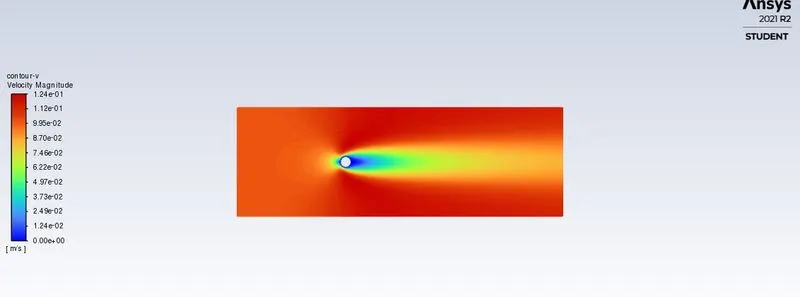
Video plot for Contour Velocity:

Pressure Contour:

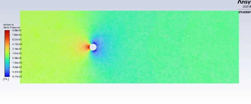
Coefficient of lift:

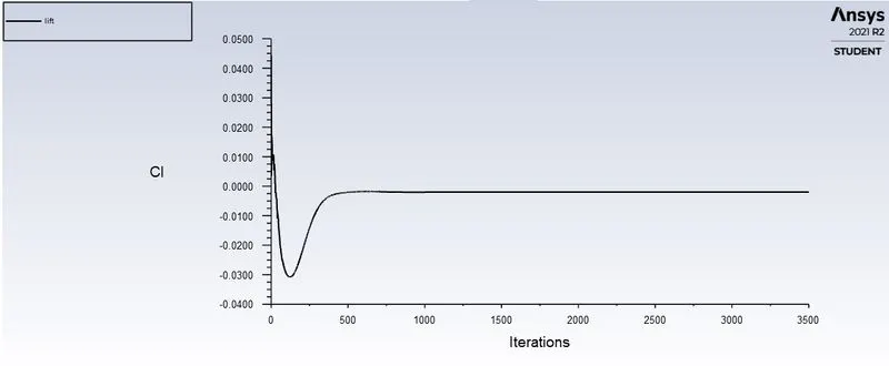
Coefficient of Drag:

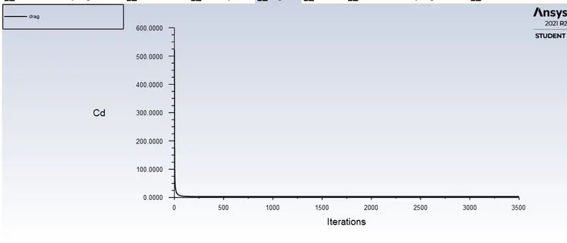
Cd-wall 3.3259448

Reynolds Number =100

Residual Plots:

Vertex Average for Velocity plot:

Velocity Contour:

Video Plot for the Contour Velocity:

Coefficient of lift:

Coefficient of Drag:

Cd-wall 1.3128797

Pressure Contour:

Reynolds Number=1000

Residual plot:

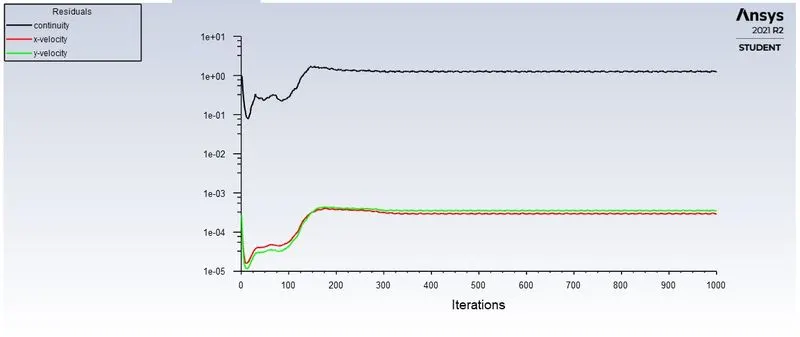
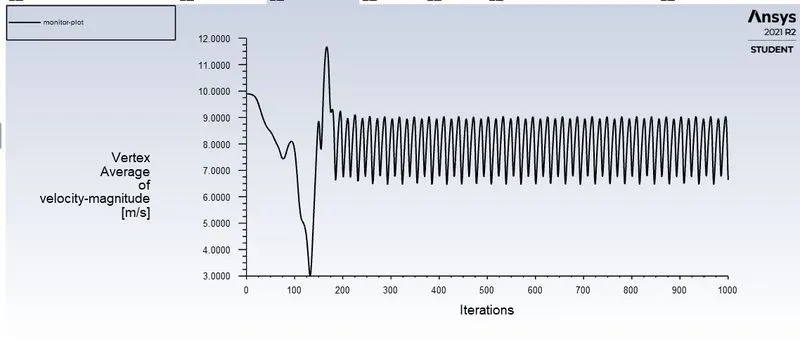
Vertex Average of Velocity:

Velocity Contour:

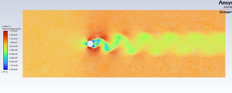
Velocity Video:

Coefficient of lift:

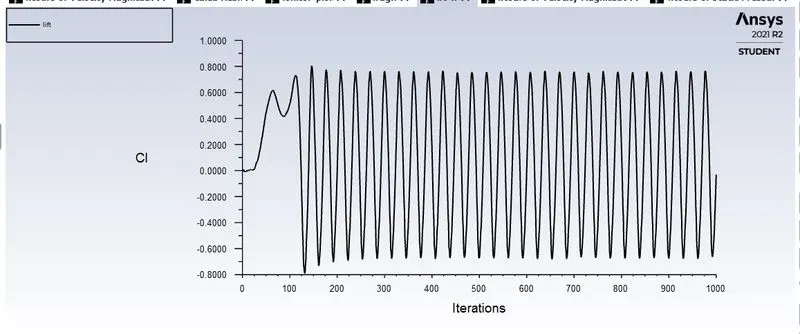
Coefficient of drag:

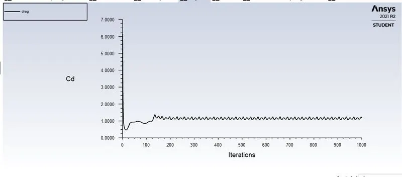
Cd-1.27760167

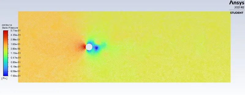
Pressure Contour:

Reynolds Number = 10000

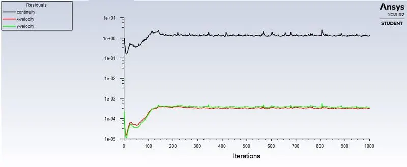
Residual Plot:

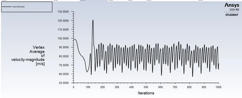
Vertex Average Velocity Plot:

Velocity Contour:

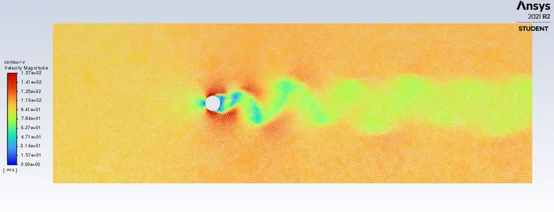
Velocity Contour Video:

Coefficient of drag:

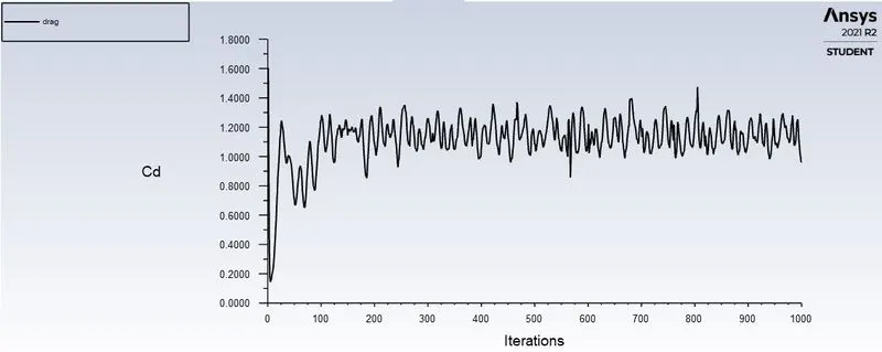
Cd-wall 0.927601637

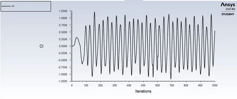
Coefficient of lift:

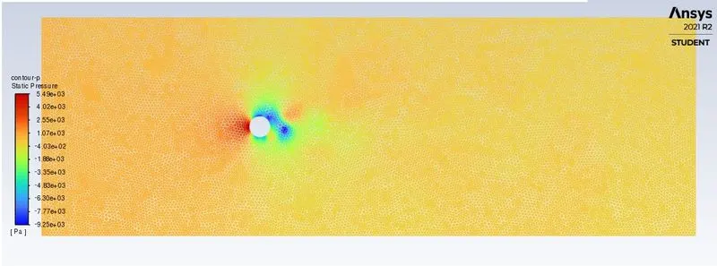
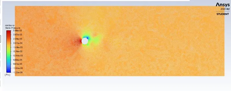
Pressure Contour:

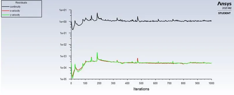
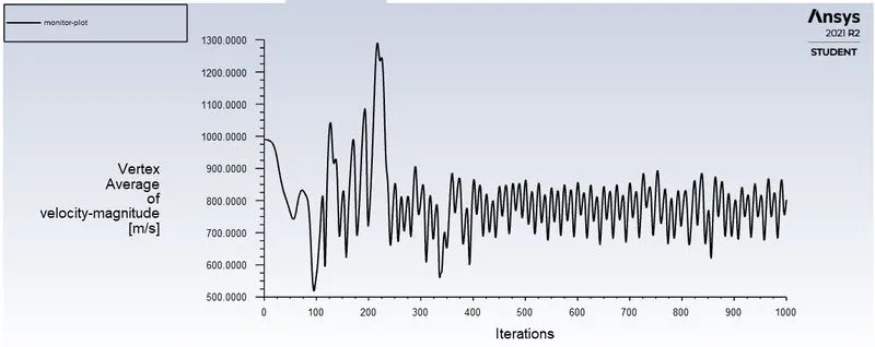
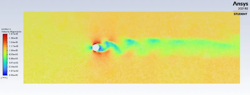
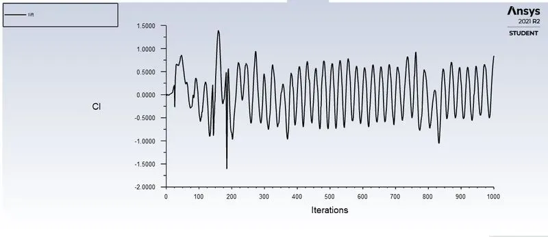
Reynolds Number = 100000

Residual Plot:

Vertex Average Velocity Plot:

Velocity Contour:

Velocity Contour Video:

Coefficient of drag:

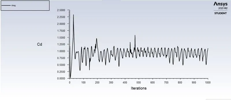
Cd-wall 1.057601637

Coefficient of lift:

Pressure Contour:

Result and Discussion:

Coefficient of Drag Numerical vs Experimental Calculation:

Reynolds Number	Coefficient of Drag(Numerical)	Coefficient of Drag(Experimental)	Percentage Absolute Difference
10	3.3259448	3.3553	2.935
100( Steady)	1.3128797	1.3475	3.492
100(Unsteady)	1.3686412	1.3475	2.114
1000	1.2776754	1.1939	8.3775
10000	0.9260176	1.0286	10.25824
100000	1.0576784	0.9537	10.39784

• Experimental Values of Coefficient of Drag are taken from the Wieselberger (1922).
• The Reynolds number increases with a Decrease in Coefficient of Drag and Increases with the Coefficient of lift.

Conclusion:

• In both cases, the solution converged is identified with the Drag and lift plots.

References:

• DEVELOPED LAMINAR FLOW IN PIPE USING COMPUTATIONAL FLUID DYNAMICS by M. Sahu [et]
• Wieselsberger, on the drag of circular cylinders, Physikalische Zeitschrift, vol. 22, 1992, pp. 219–224
• http://www.fem.unicamp.br/~phoenics/SITE_PHOENICS/AULAS/TURBULENCE/TURBULENT%20DEVELOPING%20FLOW%20IN%20A%20PIPE/pipe_developing_tutorial%20fluent.pdf