Week - 2 - Explicit and Implicit Analysis
AIM :
To Solve using both Explicit and Implicit methods using the F(u) = u3+9u2+4u equation.
THEORY :
Explicit Method :
However, if the nonlinear force versus displacement relationship is not known, but the stiffness is known, it is possible to construct the graph of force versus displacement numerically. One method is to use an incremental explicit load control scheme. This is illustrated next. For this example, three equal load increments (or steps) of ∆F = 1 unit each are used to load the tension bar. The variables used are u for displacement, f for internal force in the bar, F for the external force applied to the bar, and k for stiffness. Incremental displacements or incremental externally applied forces are represented as ∆u or ∆F, respectively. Use is made of the relationship ∆F = k∆u.
Implicit Method :
An implicit analysis is the same as an explicit analysis, except that at the end of each step Newton-Raphson iterations are used to enforce equilibrium before moving to the next step. Basically, an incremental force is applied to advance the solution forward at the beginning of a step. However, internal forces and external forces will not be in equilibrium unless the stiffness is linear for the given step. Hence, in order to achieve equilibrium, corrections must be made to the displacement. This is accomplished by using Newton-Raphson iterations to minimize the residual, `R(u)=f_i-F_e`. Expanding the residual as a Taylor series about the current displacement 'u^j' gives
`R^(j+1)=R^j(u^j)+((dR(u^j))/(du))deltau^(j+1)+...=R^j+K(u^j)(deltau^(j+1))+....`
By neglecting higher-order terms in the series, setting Rj+1 = 0, and solving for δuj+1 the following correction is obtained
`deltau^(j+1)=-[K(u^j)]^-1*R^j`
Notice that the iteration variable is j and it may take several iterations for the norm of the residual, Krk, to be reduced below the chosen tolerance criteria (for the example below a tolerance of 10−2 is chosen). The implicit analysis proceeds as follows (results are approximate, they are more precise if done in a computer to machine precision).
PROCEDURE :
Given :
Explicit Method :
`F(u) = u^3 + 9u^2 + 4u`...........eqn(1)
From eqn(1) it follows the Stiffness of the bar,
`K(u) = (df)/(du)`
`K(u) = 3u^2+18u+4`
Step-1 :
`u_0 = 0.0`, `K(u_0)=4`, `triangleF_1=1`,
`triangleu_1 = (triangle F_1)/(K(u_0))=0.25`
`u_1=u_0+triangleu_1=0+0.25`
`u_1=0.25`
Step-2 :
`K(u_1) = 3u^2+18u+4`
`K(u_1) = 0.1875+4.5+4`
`K(u_1) = 8.6875`
`triangleF_2=1`,
`triangleu_2 = (triangle F_2)/(K(u_1))=1/8.6875 = 0.115`
`u_2=u_1+triangleu_2 = 0.25+0.115`
`u_2=0.365`
Step-3 :
`K(u_2) = 3u^2+18u+4`
`K(u_2) = 0.399+6.57+4`
`K(u_2) = 10.969`
`triangleF_3=1`,
`triangleu_3 = (triangle F_3)/(K(u_2))=1/10.969 = 0.0911`
`u_3=u_2+triangleu_3 = 0.25+0.115`
`u_3=0.4561`
External & Internal Force Calculation :
`F_(e) = triangleF_1+triangleF_2 + triangleF_3 = 3`
`f_(i1) = u_1^3+9u_1^2+4u_1`
= 0.0156 + 0.5625 + 1
`f_(i1) = 1.5781`
`f_(i2) = u_2^3+9u_2^2+4u_2`
= 0.0486+1.199+1.46
`f_(i2) = 2.7076`
`f_(i3) = u_3^3+9u_3^2+4u_3`
= 0.0948 + 1.871 + 1.824
`f_(i3) = 3.7898`
Summary of Explicit analysis results :
| Step i | `triangleF_i` | `triangleu_i` | `u_i` | `(F_e)_i` | `(f_i)_i` | `f_i-F_e = R` |
| 1 | 1 | 0.25 | 0.25 | 1 | 1.5781 | 0.5781 |
| 2 | 1 | 0.115 | 0.365 | 2 | 2.7076 | 0.7076 |
| 3 | 1 | 0.0911 | 0.4561 | 3 | 3.7898 | 0.7898 |
Implicit Method :
`F(u) = u^3 + 9u^2 + 4u`...........eqn(1)
From eqn(1) it follows the Stiffness of the bar,
`K(u) = (df)/(du)`
`K(u) = 3u^2+18u+4`
Step-1 :
`u_0 = 0.0`, `K(u_0)=4`, `triangleF_1=1`,
`triangleu_1 = (triangle F_1)/(K(u_0))=0.25`
`u_1=u_0+triangleu_1=0+0.25`
`u_1=0.25`
Check the residual
`F_e=triangleF=1,`
`f_i = u_1^3+9u_1^2+4u_1`
= 0.015625+0.5625+1
`f_i = 1.578125`
`R^0=f_i-F_e=0.578125`
`||R^(0)||>10^-2` - Newton-Raphson iterations are necessary.
Calculate the correction to `u_1 = u_1^(0)`
`deltau^(1) =-[K(u_1^(0))]^-1*R^0`
`deltau^(1) =-(8.6875)^-1*0.578125`
`deltau^(1) = -0.06654`
The updated value of`u_1^(1) = u_1^(0) + deltau^(1)`
`u_1^(1) = 0.25-0.06654`
`u_1^(1) = 0.18346`
Check the residual again, `F_e=1`,
`f_i = (u_1^(1))^3+9(u_1^(1))^2+4(u_1^(1))`
= 0.0062+0.303+0.73384
`f_i = 1.04304`
`R^(1)=f_i-F_e`
`R^(1)= 1.04304-1`
`R^(1)= 0.04304`
`||R^(1)||>10^-2` - Another Newton-Raphson iterations are necessary.
Calculate the new total correction to `u_1 = u_1^(0)`
`deltau^(2) = deltau^(1) - [K(u_1^(1))]^-1*R^1`
`deltau^(2) = -0.06654 - (7.40318)^-1*0.04304`
`deltau^(2) = -0.0723`
The updated value of`u_1^(2) = u_1^(1) + deltau^(2)`
`u_1^(2) = 0.25-0.0723`
`u_1^(2) = 0.1777`
Check the residual again, `F_e=1`,
`f_i = (u_1^(2))^3+9(u_1^(2))^2+4(u_1^(2))`
= 0.0056+0.282+0.7108
`f_i = 0.9984`
`R^(2)=f_i-F_e`
`R^(2)= 0.9984-1`
`R^(2)= -0.0016`
`||R^(1)||<10^-2` - No further iterations are necessary.
Therefore the final value of `u_1=u_1^(2) = 0.1777`
Step-2 :
`K(u_1) = 3u^2+18u+4`,
`K(u_1) = 0.0947+3.1986+4`,
`K(u_1) = 7.2933`,
`triangleF_2=1`,
`triangleu_2 = (triangle F_2)/(K(u_1))=0.1371`
`u_2=u_ 1+triangleu_2=0.1777+0.1371`
`u_2=0.3148`
Check the residual
`F_e=triangleF=2,`
`f_i = u_2^3+9u_2^2+4u_2`
= 0.0312+0.8918+1.2592
`f_i = 2.1822`
`R^0=f_i-F_e= 0.1822`
`||R^(0)||>10^-2` - Newton-Raphson iterations are necessary.
Calculate the correction to `u_2 = u_2^(0)`
`K(u_2) = 3u^2+18u+4`
= 0.2972+5.6664+4
`K(u_2) = 9.9636`
`deltau^(1) =-[K(u_2^(0))]^-1*R^0`
`deltau^(1) =-(9.9636)^-1*0.1822`
`deltau^(1) = -0.0183`
The updated value of`u_2^(1) = u_2^(0) + deltau^(1)`
`u_2^(1) = 0.3148-0.0183`
`u_2^(1) = 0.2965`
Check the residual again, `F_e=1`,
`f_i = (u_2^(1))^3+9(u_2^(1))^2+4(u_2^(1))`
= 0.0260+0.7912+1.186
`f_i = 2.0032`
`R^(1)=f_i-F_e`
`R^(1)= 2.0032-2`
`R^(1)= 0.0032`
`||R^(1)||<10^-2` - No further iterations are necessary.
Therefore the final value of `u_2=u_2^(1) = 0.2965`
Step-3 :
`K(u_2) = 3u^2+18u+4`,
`K(u_2) = 0.2637+5.337+4`,
`K(u_2) = 9.6007`,
`triangleF_2=1`,
`triangleu_3 = (triangle F_2)/(K(u_2))=0.1041`
`u_3=u_ 2+triangleu_3=0.2965+0.1041`
`u_3=0.4006`
Check the residual
`F_e=triangleF=3,`
`f_i = u_3^3+9u_3^2+4u_3`
= 0.0643+1.4443+1.6024
`f_i = 3.111`
`R^0=f_i-F_e= 0.111`
`||R^(0)||>10^-2` - Newton-Raphson iterations are necessary.
Calculate the correction to `u_3 = u_3^(0)`
`K(u_3) = 3u^2+18u+4`
= 0.4814+7.2108+4
`K(u_3) = 11.6922`
`deltau^(1) =-[K(u_2^(0))]^-1*R^0`
`deltau^(1) =-(11.6922)^-1*0.111`
`deltau^(1) = -0.0095`
The updated value of`u_3^(1) = u_3^(0) + deltau^(1)`
`u_3^(1) = 0.4006-0.0095`
`u_3^(1) = 0.3911`
Check the residual again, `F_e=1`,
`f_i = (u_3^(1))^3+9(u_3^(1))^2+4(u_3^(1))`
= 0.0598+1.3766+1.5644
`f_i = 3.0008`
`R^(1)=f_i-F_e`
`R^(1)= 3.0008-3`
`R^(1)= 0.0008`
`||R^(1)||<10^-2` - No further iterations are necessary.
Therefore the final value of `u_3=u_3^(2) = 0.3911`
Summary of Implicit analysis results :
| Step i | `triangleF_i` | `u_i` | `(F_e)_i` | `(f_i)_i` | `f_i-F_e = R` |
| 1 | 1 | 0.1777 | 1 | 0.9984 | -0.0016 |
| 2 | 1 | 0.2965 | 2 | 2.0032 | 0.0032 |
| 3 | 1 | 0.3911 | 3 | 3.0008 | 0.0008 |
Exact Solution by solving third order Polynomial :
`F(u) = u^3 + 9u^2 + 4u`
`u^3 + 9u^2 + 4u - F(u) = 0`
| Step i | `(F_e)_ i` | `u_i` |
| 1 | 1 | 0.17762 |
| 2 | 2 | 0.29616 |
| 3 | 3 | 0.39103 |
Plot Results :
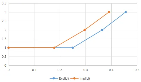
(i) Comparison of Force vs Displacement of Implicit and Explicit method :
(ii) Comparison of Force vs Displacement of Explicit, Implicit and Exact solution method :
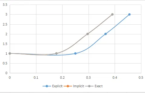
From the above plots, we obtained that the Implicit method gives a better solution comparing with the Explicit method. The implicit method will be equal to the exact solution due to Newton Raphson iterations used to enforce the equilibrium of external & internal forces.