Week - 2 - Explicit and Implicit Analysis

Aim : To study the differences between implicit and explicit analyses.

Procedure : The comparsion is made between implicit and explicit analyses as follows.

Implicit Analysis	Explicit Analysis
It is independent of time.	It is dependent on time.
Implicit analysis is unconditionally stable.	Explicit analysis is stable only on the condition that that the timestep is lesser than the time required for a soundwave to travel between two nodes of an element.
There is no K matrix inversion.	There is K matrix inversion.
Timestep size is kept larger.	Timestep size is kept smaller.
Accuracy is the limiting factor for timestep.	Stability is the limiting factor for timestep.
It has a larger cost per timestep due to more complex calculations.	It has a smaller cost per timestep due to lesser calculations.
Equilibrium is ensured throughout the simulation and is maintained at every timestep which requires more calculations.	Equilibrium is not maintained at every timestep and as a result of this the simulation goes on computing, hence smaller timestep is the only way to ensure stability.
Parallel processing is possible.	Parallel processing is not possible.
It is used in slow speed, fatigue type simulations with constant loading or loading over a large period of time.	It is used in dynamic simulations such as crash analysis, impact analysis etc where the crash occurs over a very small time period.
This method is used to perform the analysis on cases where the strain rate does not affect the method of deformation.	This method is used to perform the analysis on cases where the strain rate affects the method of deformation.

Part 2 : Mathematical differences of explicit and implicit analysis.

Equation		Constants
Fint	u³+9u²+4u	ΔF = 1
Stiffness(k)	1 + u²	ΔUn = ΔF/kn-1
Correction (ẟu)	(-[k(ui)^-1*R])
Explicit Analysis (i)	u0	k0	Δu	u0 + Δu = ui	Fext	Fint	Fint-Fext = R
Step1	0	1	1	1	1	14	13
Step2		2	0.5	1.5	2	29.625	27.625
Step3		3.25	0.308	1.808	3	42.562	39.562

For the following equation given in the question the explicit analysis is performed as follows. As we can see, due to the equation of force, there is a large difference between external and internal force if an external force of ΔF = 1 is taken for every increment.

ui = total displacement after adding ΔU

Fext = ΔF = 1 getting added at every step

Fint = force calculated by substituting value of ui in eqn for Fint.

R = correction required ( Fint - Fext)

This is what happens in implicit analysis when a correction factor is applied at every step to make the internal force equal to the external force of ΔF = 1. In this analysis, the correction factor comes into play.

Implicit Analysis (i)	u0	k0	Δu	u0 + Δu = ui	Fext	Fint	Fint-Fext = R	ẟui ( correction)
Step1	0	1	1	1	1	14	13	-6.5
				-5.5	1	105.88	104.88	-3.356
				-8.856	1	-24.129	25.129	-0.3164
				-9.1724	1	-51.194	52.194	-0.613

ẟui = correction factor (-[k(ui)^-1*R])

As we can see, the calculated value Fint is very irregular and keeps increasing and decreasing in comparison to Fext. Due to this correction factor calculated ẟui keeps giving a a value for ui that keeps getting further and further away from Fext. The solution is found to be diverging for this particular equation due to the fact that R never tends to be lesser than 0.001 which was required tolerance value for the question.

If we look at the equation taken in the pdf ptovided for the question.

Fint	u + u³/3
Implicit Analysis (i)	u0	k0	Δu	u0 + Δu = ui	Fext	Fint	Fint-Fext = R	ẟui (first correction)
Step1	0	1	1	1	1	1.333	0.333	-0.1665
				0.8335	1	1.0265	0.0265	-0.0156
				0.8179	1	1.0028	0.0028	nil
Step2		1.66888	0.5992	1.4171	2	2.3655	0.3655	-0.1067
				1.3104	2	2.0602	0.0602	-0.1266
				1.2904	2	2.0066	0.0066	nil
Step3	and so on..
				1.6097	3	3.000016	0.000016	nil

As we can see for the changed equation of u, the value of R keeps reducing as we iterate and this leads to the correction factor ẟui becoming nil(not required) and hence the simulation proceeds onto the next step of addition of

Fext = 1, making total Fext=2,3 and so on....

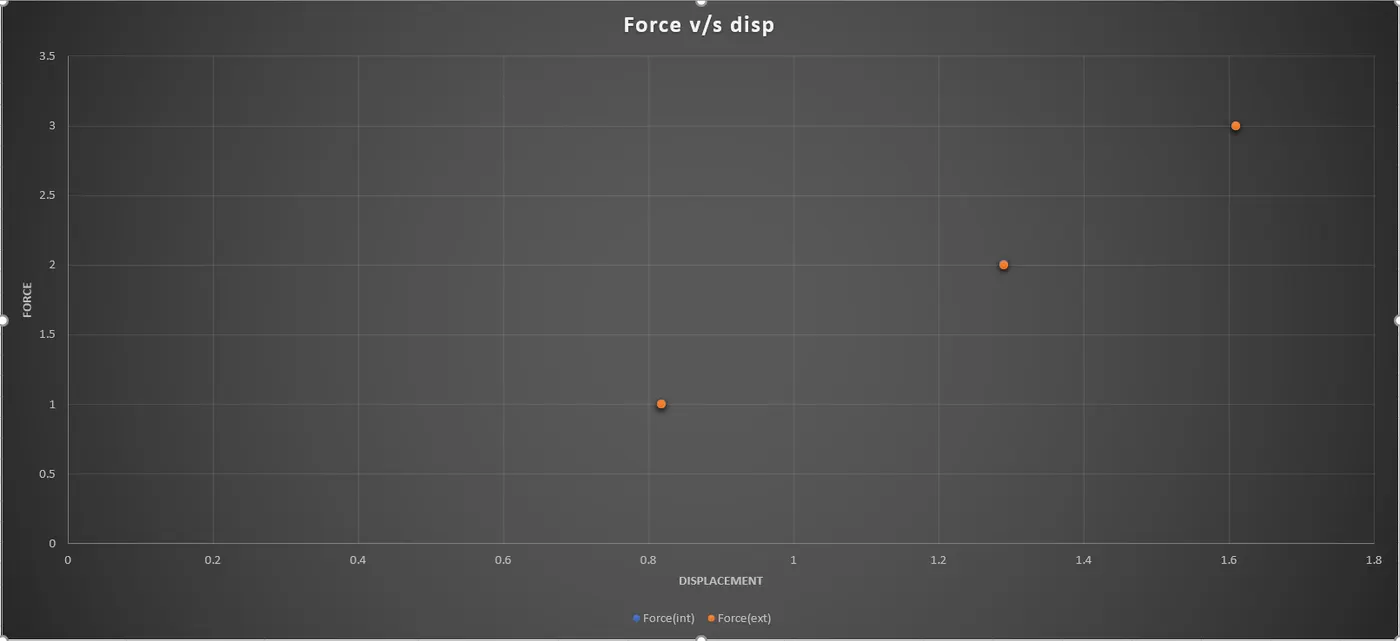
As we can see in the final iteration of each step the calculated values of Fint (in bold) are very close to the values of Fext and within the tolerance range of 0.001 .This allows the simulation to move onto the next step.

The graph is plotted for above table with exact values of force in blue dots and implicit calculated values in orange dots. We can see that they are almost coincident, hence only one colour of dots are visible in the force v/s displacment graph.

Conclusion : In earlier case the equation was not compatible with implicit analysis, or the equation of stiffness k must also be modified suitablly, or ΔF must be changed suitably, otherwise we get a diverging solution.

Result : Hence implicit vs explicit analysis has been studied in detail.