Week - 2 - Explicit and Implicit Analysis

Objective: Consider the given problem and solve it using both Explicit and Implicit method and compare with Exact solution.

F(u)= u³+9u²+4u

Aim: To understand and compare the results between Explicit and Implicit analysis and how it varies from Exact result.

Solution: We can suppose that forde in the given problem is Non-Linear function of displacement.
F(u) = u³+9u²+4u ....(1)

From (1) we can say that stiffness is
K(u) = du/df = 3u²+18u+4 ....(2)

Explicit:

From Equation (1) we can plot Force vs displacement diagram. However, the non-linear displacement relationship is not known, but stiffness is known as in Equation (2)

We can use an Incremental Explicit Load Control Scheme to find the solution,

Here,
u = displacement
F(int)= internal Force
F(ext)= External Force
K= stiffness
ΔF= Incremental Force
Δu = Incremental Displacement

We will use the relationship ΔF = KΔU

Step 1:

u0 = ,
K(u0)= 3(u0²)+ 18(u0²)+4
= 3(0) + 18(0) +4
=4
ΔF = 1

Δu1= ΔF/K(u0)
= 1/4 = 0.25
u1 = u0+Δu1
=0 + 0.25 = 0.25

F(ext) = 1
F(int) = (u1)³+ 9(u1)² + 4(u1)
= (0.25)³+ 9(0.25)² + 4(0.25)
= 1.579


Step 2:

K(u1)= 3(u1²)+ 18(u1²)+4
= 3(0.25) + 18(0.25) +4
=8.6875
ΔF = 1

Δu2= ΔF/K(u1)
= 1/8.6875 = 0.115
u2 = u1+Δu2
= 0.25+ 0.115 = 0.365

F(ext) = 1
f(int) = (u2)³+ 9(u2)² + 4(u2)
= (0.365)³+ 9(0.365)² + 4(0.365)
= 2.707

Step 3:
K(u2)= 3(u1²)+ 18(u1²)+4
= 3(0.365) + 18(0.365) +4
=10.97
ΔF = 1

Δu3= ΔF/K(u2)
= 1/10.97 = 0.091
u3 = u0+Δu1
= 0.365 + 0.091 = 0.456

F(ext)= 1
f (int) = (u3)³+ 9(u3)² + 4(u3)
= (0.456)³+ 9(0.456)² + 4(0.456)
= 3.79

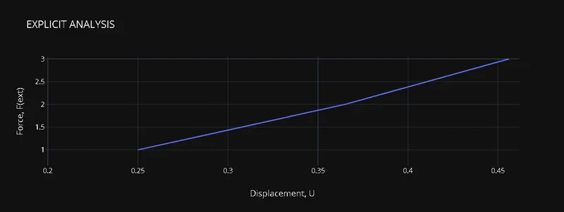
STEPS	ΔF	ΔU	U	F(ext)	F(int)	R
1	1	0.25	0,25	1	1.579	0.579
2	1	0.115	0.365	2	2.707	0.707
3	1	0.091	0.456	3	3.79	0.79

Implicit:

The Implicit method is same as the Explicit, however, Newton-Raphson iterations are required at end of each step before moving on to the next step.

However, internal and external forces will not be in equilibrium unless the stiffness is linear for given step, hence corrections must be made to displacement. This is achieved by Newton-Raphson iteration to minimize residue.

R^(i+j) = R^j(u^j)+ dR(u^j)/du. δu^j+i.........+ R^j+ K(u^j).δu^j+i+.......

By neglecting higher order terms and setting R^j+i =0 and solving for δu^j+i the following correction is obtained.

δu^j+i= -[K(u^j)]^-1. R^j


Step 1:

u0= 0,
k(u0)= 3(0)²+18(0)+4 = 4
ΔF = 1,
Δu1 = ΔF/k(u0)
= 1/4 =0.25
u1 = u0+ Δu1 = 0.25

Check for residue, R0 = F-f

F(int) = (0.25)³+9(0.25)²+4(0.25)
= 1.578
R0 = F(int)- F(ext)
= 1.578 - 1
R0 = 0.578

Since R0>10^-2 Newton-Raphson iteration is required.

Iteration 1:

Calculate the corrections to u1 = (u1)⁰

δ(u1) = -[k(u1)]^-1. (R⁰)

k(u1)⁰= 3(0.25)³+18(0.25)+ 4
= 8.6875

δ(u1) = -(8.6875)^-1. 0.578
= 0.0665

Update the value of (u1)¹ = (u1)⁰+ δ(u1)
= 0.25+ (-0.0665)
u1 = 0.1835

Check residue again,

F(ext) = 1
F(int) = (0.1835)³+ 9(0.1835)+4(0.1835)
F(int) = 1.0432

R1 = F(int)- F(ext)
=1.0432-1
= 0.0432
Since R1> 10^-2 Newton Raphson Iteration is required

Iteration 2:

Calculate the corrections to u1 = (u1)¹

δ(u2) = -[k(u1)]^-1. (R¹)

k(u1)¹= 3(0.1835)²+18(0.1835)+ 4
= 7.404

δ(u2) = -(7.404)^-1. 0.0432
= -0.0723

Update the value of (u1)¹ = (u1)⁰+ δ(u1)¹
= 0.25+ (-0.0723)
u1 = 0.1777

Check residue again,

F(ext) = 1
F(int) = (0.1777)³+ 9(0.1777)+4(0.1777)
F(int) = 1.00060

R(2) = F(int)- F(ext)
= 1.0006 - 1
= 0.0006


Since R(1) > 10^-2 further Newton-Raphson Iteration is not required.


Step 2:

u1 = 0.1777
K(u1) = 3(0.1777)²+18(0.1777)+4
= 7.2933
ΔF= 1

Δu1 = ΔF/k(u1)
= 1/7.2933
Δu2 = 0.1371

u2= Δu2 + u1
= 0.1777+ 0.137
= 0.3147

Check for residue,

R = F(int) - F(ext)
F(int) = (0.3147)³+ 9(0.3147)²+ 4(0.3147)
= 2.181
R = 2.181 - 2
= 0.181
Since R> 10^-2 Newton-Raphson iterations are required.

Calculating the corrections to u2=(u2)⁰

δ(u2) = -[K(u2)]^-1.R

K(u2) = 3.(0.3147)²+ 18(0.3147)+ 4
= 9.9617
δ(u2) = -[9.9617]^-1. (0.181)
= -0.0182
Update value at u2 =(u1⁰)+ δu2
u2 = 0.3147 - 0.0182
u2 = 0.2965

Check the residue,

R1 = F(int) - F(ext)
F(int) = (0.2965)³+ 9(0.2965)²+ 4(0.2965)
= 2.0032

R2 = 2.003-2
= 0.003

Since the R2< 10^-2, further iterations are not required.


Step 3:

u2 = 0.2965

K(u2) = 3(0.2965)²+ 18(0.2965)+ 4
K(u2) = 9.6007

Δu3 = ΔF/Ku
= 1/ 9.6007
= 0.1041

u3 = u2 + Δu3
= 0.2965 + 0.1041
= 0.4006

Check for residue
R = F(int) - F(ext)

F(int) = (0.4006)³ + 9(0.4006)² + 4(0.4006)
= 3.1110

R = 3.1110-3
= 0.110

Since R>10^-2 another Newton-Raphson iteration is required

δ(u2) = K(u2).R

K(u2) = 3(0.4006)²+18(0.4006)+4
= 11.69

δ(u2) = -[11.69]^-1 . 0.1110
= 0.0092

u3 = u2+ δ(u2)
= 0.4006 - 0.0094
= 0.3912

Check for residue again,

R = F(int)-F(ext)

F(int) = (0.3912)³+ 9(0.3912)²+4 (0.3912)

F(int) = 3.0008

R = 3.0008- 3
= 0.0008

Since R<10^-2 another iteration is not required.

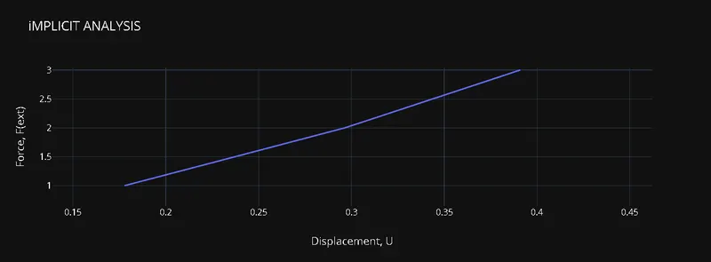
STEPS	ΔF	ΔU	U	F(ext)	F(int)	R
1	1	0.25	0,1777	1	1.006	0.006
2	1	0.115	0.2965	2	2.003	0.003
3	1	0.091	0.3912	3	3.008	0.008

Exact Solution:


Taking Third Order Polynomial of Non Linear Displacement Equation:

Take F(u) = u³+9u²+4u

F(u) = 1,
u³+9u²+4u-1 = 0,
This Equation is solved using Scientific Calculator with Polynomial Degree 3,
u1 = 0.1776

F(u) = 2,
u³+9u²+4u-2 = 0,
This Equation is solved using Scientific Calculator with Polynomial Degree 3,
u2 = 0.2961


F(u) = 3,
u³+9u²+4u-3 = 0,
This Equation is solved using Scientific Calculator with Polynomial Degree 3,
u3 = 0.3911


IMPLICIT VS EXPLICIT

There are two ways in which a model discretization can be done:

Spatial Discretization

Time Discretization

Spatial Discretization is where the model with infinite DOF is converted into a model into FINITE ELEMENT and DOF.

Time Discretization is in which method one has to solve the physical problems that are provided. This is where Explicit and Implicit time integration comes into play.

IMPLICIT METHOD:

In Implicit Analysis, unknown terms in the equation are solved through matrix inversion. In Implicit Analysis generally, the effect of mass/inertia is neglected. When the problem is Non-Linear solution of each step requires a series of trial solutions (iterations) to establish equilibrium within a certain tolerance. It requires a numerical solver to invert a numerical matrix once or even several times. These solutions are unconditionally stable & facilitate large-time steps. Despite these advantages, the Implicit Method can be extremely time-consuming when solving dynamic & non-linear problems.

EXPLICIT METHOD:

Explicit Analysis aims to solve for acceleration. In most cases, the mass matrix is considered as lumped and thus a diagonal matrix. The increase of the diagonal matrix is straightforward and includes the terms on the diagonal only. Once the acceleration is calculated at (N)th step, velocity at N1/2 step and displacement at N+1 step are calculated accordingly. This method is not Unconditionally Stable hence smaller time step is required. It requires a time-step to be smaller than CFL(Courant Friedrich Levy) Criteria.

Time Step, ΔT = Lc/C

where,

Lc = Characteristic length of the meh

C = Speed of sound wave through the element (material)

Difference between Implicit and Explicit Analysis:

	IMPLICIT	EXPLICIT
Deformation	Small	Large
What Causes Large Deformation	Pure Force, Dynamics	Velocity, Acceleration, with mass/inertia
K- Matrix Inversion	Yes	No
TIme-Step Size	Large	Small
Cost Per TIme STep	Large	Large
Cost Increase for Doubling	X128	X16

COMPARISON SOLUTIONS OF EXPLICIT, IMPLICIT METHODS AND EXACT SOLUTIONS:

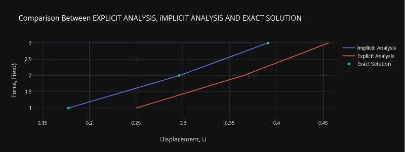
From the graph, we can see that the Implicit Solution is same as the Exact Solution, whereas the Explicit solution is comparatively less accurate. However, despite having more accurate results Implicit solution can be preferred over Exact Solution in all conditions, as it more time-consuming.

CONCLUSION: From the results above and the explanation we can conclude that Implicit Method is accurate to the exact solution. However, it is more time-consuming and requires much smaller whereas in Explicit we can have larger time-step and element size. Hence, we can say that we can decide the Solving method based on the physics and type of analysis required for a particular model.