Week - 2 - Explicit and Implicit Analysis
F(u) = u3+9u2+4u the equation was solve by using both Explicit and Implicit Methods.
1. Write a detailed report about Implicit and explicit methods.
2. Caliculations was done practice book and same formulas was utilized to solve this problem according to that information graphs are represented in attached document.
IMPLICIT & EXPLICIT PROBLEM
Introduction:-
This article illustrates a nonlinear static problem. An explicit and implicit analysis is used to
solve the problem. An incremental load control scheme is used in both cases.
The example as presented is clearly fabricated. Some aspects of this exercise may appear
strange to a beginner. The example problem, on the other hand, is designed to demonstrate a
variety of concepts that may arise in a typical nonlinear finite element analysis. It is beneficial to
consider This exercise provides some basic tools that will be useful in the future..
Problem:-
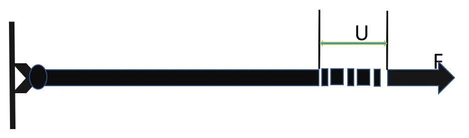
Consider the case of a simple bar in tension as shown in Figure 1. Suppose that the
force in the bar is a nonlinear function of the displacement f(u) = U^3+9U^2+4^U ----------------------------(1)
From (1) it follows that the stiffness of the bar is k(u) =3U^2+18^U+4 -----------------------------(2)
Explicit Analysis
Clearly it is possible to plot a graph of force, f, versus displacement, u, by using equation
(1) (see Figure 2). However, if the nonlinear force versus displacement relationship is
not known, but the stiffness is known, it is possible to construct the graph of force versus
displacement numerically. One method is to use an incremental explicit load control scheme.
This is illustrated next. For this example three equal load increments (or steps) of F = 1
unit each are used to load the tension bar. The variables used are u for displacement, f for
internal force in the bar, F for external force applied to the bar and k for stiffness. Incremental
displacements or incremental externally applied forces are represented as u or F,
respectively. Use is made of the relationship F = ku. The analysis proceeds as follows:
2
Step 1
u0 = 0.0, ⇒ k(u0) = 4, F = 1, u1 = F/k(u0) = 1/4, u1 = u0 + u1 = 0.25
Step 2
⇒k(u1) = 3(0.25)2+18(0.25)+4 = 8.687 , F = 1, u2= F/k(u1) = 1/8.687, u2= u1+ u2= 0.365
Step 3
⇒ k(u2) =3(0.365)2+18(0.365)+4 = 10.969, F = 1, u3= F/k(u2) = 1/10.969, u3= u2+u3∼=11
Finally, from the three steps the following results are obtained.
Fext= F + F + F = 3.0
fint= Ui3+9Ui2+4Ui , U1=0.25,(0.25)^3+9(0.25)^2+4(0.25) = 1.57
U2=0.365, (0.365)^3+9(0.365)^2+4(0.365) = 2.707,U3=0.456, (0.456)^3+9(0.465)^2+4(0.456) = 3.790
The results show that external and internal forces are not in equilibrium because Fext does not equal Fint. Table
1 summarizes the main findings from the explicit analysis.
Table 1: Summary of explicit analysis results
| Step i | Fi | ui | ui | (Fext)i | (fint)i | fint − Fext = R |
| 1 | 1.0 | 0.25 | 0.25 | 1.0 | 1.57 | 0.57 |
| 2 | 1.0 | 0.115 | 0.365 | 2.0 | 2.707 | 0.707 |
| 3 | 1.0 | 0.0119 | 0.456 | 3.0 | 3.790 | 0.790 |
Implicit Analysis
An implicit analysis is the same as the explicit analysis, except that at the end of each step
Newton-Raphson iterations are used to enforce equilibrium before moving to the next step.
Basically, an incremental force is applied to advance the solution forward at the beginning
of a step. However, internal forces and external forces will not be in equilibrium unless the
stiffness is linear for the given step. Hence, in order to achieve equilibrium, corrections must
be made to the displacement. This is accomplished by using Newton-Raphson iterations to
minimize the residual, R(u) = fint − Fext. Expanding the residual as a Taylor series about
the current displacement uj gives
Rj+1 = Rj(uj) +dR(uj)du
uj+1 + ... = Rj + k(uj)uj+1 + ... (3)
3
By neglecting higher order terms in the series, setting Rj+1 = 0 and solving for uj+1 the
following correction is obtained
uj+1 = −[k(uj)]−1Rj . (4)
Notice that the iteration variable is j and it may take several iterations for the norm of the
residual, kRk, to be reduced below the chosen tolerance criteria (for the example below a tolerance
of 10−2 is chosen). The implicit analysis proceeds as follows (results are approximate,
they are more precise if done in a computer to machine precision):
Step 1
u0 = 0.0,⇒ k(u0)=4,F = 1,u1= F/k(u0) = 1/4 ,u1 = u0 + u1 =0.25 Check
the residual, Fext = F = 1, fint = U1^3+9U1^2+4^U=1.578, R(0) = fint − Fext =0.578
R(0)>10−2 ⇒ Newton-Raphson iterations are necessary.
Calculate the correction to u1 = u1
(0)
u(1) = −[k(u1
(0))]−1R(0) = −8.687−1(0.578) = −0.066.
⇒ The updated value of
u1(1)= u1
(0)+ u(1)= 0.25 + (−0.066) = 0.184. Check the residual
again, Fext= 1, fint= (0.184)3+9(0.184)2+4(0.184) = 1.046.
II R(1) II= fint − Fext = 0.046.
II R(1)II > 10−2 ⇒ another Newton-Raphson iteration is necessary.
Calculate the new total correction to u1=u1(0)
u(2)= u(1)− [k(u1
(1))]−1R(1)= −0.66 − (7.413−1)0.046 = −0.072.
The updated value of u1(2)= u1
(0)+ u(2)= 0.25+ (−0.072) = 0.17. R
Check the residual, Fext= 1, fint= (0.17)3+9(0.17)2+4(0.17)= 0.94501.
R(2)= fint − Fext = -0.054
R(2)< 10−2 ⇒ no further iterations are necessary.
Therefore, the final value is u1 = u1(2) = 0.17.
Step 2
k(u1) = 3(0.17)2+18(0.17)+4= 7.146, F = 1, u2= F/k(u1) = 0.139.
u2 = u1 + u2 = 0.389
Check the residual, Fext = F = 1, fint = (0.389)3+9(0.389)2+4(0.389) = 2.976.
IIR(0)II = fint− Fext= 0.976
II R(0) II > 10−2⇒ Newton-Raphson iterations are necessary.
Calculate the correction to u2 = u2(0)
u(1) = −[k(u2
(0))]−1R(0) = −10.969−1(0.976) = −0.0889.
⇒ The updated value of u2(1) = u2
(0) + u(1) = 0.389 + (−0.0889) = 0.3001.
4
Check the residual again, Fext= 1, fint= (0.3001)3+9(0.3001)2+4(0.3001)= 2.0379
R(1) = fint − Fext = 2.0379-2=0.0397.
R(1)> 10−2 ⇒ another Newton-Raphson iteration is necessary.
Calculate the new total correction to u2 = u2(0)
u(2) = u(1) − [k(u2(1))]−1R(1) = −0.0889 − (9.67−1)0.379 = −0.09281.
The updated value of u2(2)= u2
(0)+ u(2)= 1.389 + (−0.09280) = 0.29619.
Check the residual, Fext= 1, fint= (0.29619)3+9(0.29619)2+4(0.29619) = 2.00030
R(2) = fint − Fext = 2.00030-2=0.00030
R(2)< 10−2 ⇒ no further iterations are necessary.
Therefore, the final value is u2 = u2(2) = 0.29619.
Step 3
is completed similar to steps 1 and 2, the final value is u3 = 0.382408.
The results of the implicit analysis are summarized in Table 2. It is evident from the table
that the external forces and internal forces are coming into equilibrium.
Table 2: Summary of implicit analysis results
| Step i | Fi | ui | (Fext)i | (fint)i | fint − Fext = R |
| 1 | 1.0 | 0.17 | 1.0 | 1.94501 | 0.054 |
| 2 | 1.0 | 0.29619 | 2.0 | 2.00030 | 0.000030 |
| 3 | 1.0 | 0.382408 | 3.0 | 2.90167 | 0.098 |
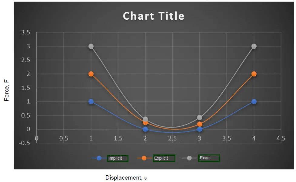
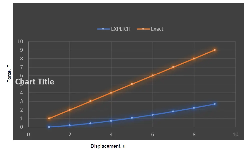
Figure 2a depicts a plot of the results. The plot clearly shows that the explicit analysis
deviates from the exact solution. The explicit analysis follows the exact solution when nine
increments are used, as shown in Figure 2b. Even with larger increments, the explicit analysis
deviates from the exact solution. The deviation from the exact solution demonstrates the
lack of balance between internal and external forces. An implicit analysis is required to correct
for this issue. Figure 2a depicts the results of the implicit analysis. Newton-Raphson iterations
correct the incremental steps until they arrive at the exact solution within the specified
tolerance. Excellent agreement is obtained with only three increments, and in each increment
(a)
(b)
Figure 2: Single bar in tension: (a) Comparison of explicit, implicit and exact results of load
versus displacement; (b) explicit results using 9 increments.
Discussion :-
In practise, when addressing large structures with numerous degrees of freedom, a more
complex convergence criterion might be required. Nonetheless, reduction of the residual
norm is a sufficient criterion for this example. It's crucial to understand how the initial increment
brought on by the incremental load progresses the solution. After that, Newton-Raphson
iterations are performed to adjust the displacement in order to attain equilibrium if an
implicit analysis is applied. A new load increment is added to progress the solution after a
suitable equilibrium has been reached, and the process is then repeated. Keep in mind that
the exact relationship between force and displacement is not always clear. Later, there will
be more discussion, including which is better: explicit or implicit? When ought I to use explicit
rather than implicit? What application does this example have to nonlinear structure
issues with multiple degrees of freedom? How big of an increment should be used in explicit?
What kind of increment size should be used for implicit? The increment's size could have an
impact on convergence speed. The Newton-Raphson iterations converge quadratically if the
increment size is appropriate. Keep in mind how the Newton-Raphson iterations update the
correction δu. Only once the equilibrium requirements have been met are the initial predicted
displacements for the given step updated with the final δu. How much tolerance is
needed to maintain equilibrium? More to come...
Conclusion:-
Incremental explicit and implicit approaches are used to illustrate a nonlinear analysis.
For comparison, the results are plotted. The findings make it clear that the explicit analysis
strays from the correct answer. This issue is solved by employing an implicit analysis that
uses Newton-Raphson iterations to ensure that internal and exterior forces are in equilibrium.
The load control scheme's strategies are illustrated. The reader is directed to the references
provided below for information on various systems such as displacement control, arc
length control, and generalised displacement control. The concepts and techniques that are
introduced resemble many of the concepts and techniques utilised in nonlinear finite element
analysis. The provided example is therefore a helpful teaching tool for students learning
about approaches to tackling nonlinear issues.
References:-
1.Crisfield, M. A. (1991). Non-linear Finite Element Analysis of Solids and Structures Vol 1.
Chichester, England: John Wiley & Sons Ltd.
2.M. J. Clarke and G. J. Hancock. A study of incremental-iterative strategies for non-linear
analyses. International Journal for Numerical Methods in Engineering, 29:1365-1391, 1990.
3.Y. B. Yang, L. J. Leu, and Judy P. Yang, Key Considerations in Tracing the Postbuckling
Response of Structures with Multi Winding Loops, Mechanics of Advanced Materials and
Structures, 14:175-189, 2007.
4.McGuire, W., Gallagher, R. H., and Ziemian, R. D., Matrix structural analysis, 2nd Ed.,
Wiley, New York, 2000.
Note:- Same content was was documented in PDF format and consider as reference and proceed grading accordingly.