Week - 2 - Explicit and Implicit Analysis
AIM:
To solve the equation F(u)=u3+9u2+4u">F(u)=u3+9u2+4uF(u)=u3+9u2+4u using both explicit and implicit methods with a residual tolerance of 0.01.
In the equation, F-Force in the bar and u-displacement in the bar.
The problem is solved by both explicit and implicit analysis methods.
In both cases an incremental load control scheme is used.
We will use Implicit and Explicit solvers to solve dynamic problems.
Implicit and Explicit analysis differ in the approach to time increments..
Overview on Explicit and Implicit analysis:
In Implicit analysis each time increment has to converge, but we can set pretty long time increments. Explicit on the other hand doesn’t have to converge each increment, but for the solution to be accurate time increments must be super small.
In general, when we want to solve a dynamic problem, we are asking the solver to calculate the series of time increments, to see what is going on in the model. In each of those increments, time slightly increases. This of course also changes the load in the model. This is why we need to have a time-dependent chart for load. So the solver knows what load should be applied at which time increment.
To this extent, it works the same as load increment in static analysis. Also, since we are incrementing time, inertia effects can be taken into account when things are happening fast enough.
To this extent, both implicit and explicit analysis does more or less the same thing. They divide the analysis time into small increments, and then analyze what is going on in our model one increment of time after another.
Explicit analysis:
Explicit analysis works in a way, that we don’t have to converge each step. There are no convergence criteria to check and no iterations.
Instead of verifying the global equilibrium, solver assumes that the equilibrium simply exists.This means that the solver goes straight into calculation of local finite element variables.It calculates all of the local finite element variables for given increment, and moves to the next one.
Time increment in explicit analysis is very short. It’s the time in which an elastic wave (i.e. impact wave) can travel through a single finite element of your model. Of course, this is verified for all finite elements in your model, and the smallest time is selected.
Implicit analysis:
Implicit analysis works in a way,that in each time increment, the global equilibrium in the model is established. This means that each increment has to converge (this is happening in iterations).
Since global equilibrium is verified at each time increments, those increments can be large.Each time increment computes slowly, since iterations are needed to get to the global equilibrium.
Explicit scheme:
If the nonlinear force versus displacement relationship is not known, but the stiffness is known, it is possible to construct the graph of force versus displacement numerically.
It can be done using an incremental explicit load control scheme.
The following equation is solved using explicit method as follows,
F(u)=u3+9u2+4u">F(u)=u3+9u2+4uF(u)=u3+9u2+4u
Differentiating force with respect to displacement gives the stiffness(k) of the bar (since F = kx).
k(u)=dFdu=3u2+18u+4">k(u)=dFdu=3u2+18u+4k(u)=dFdu=3u2+18u+4
Here,three equal load increments (or steps) of ΔF=1">ΔF=1ΔF=1 unit each are used to load the tension bar.
The variables used are u for displacement, f for internal force in the bar, F for external force applied to the bar and k for stiffness. Incremental displacements or incremental externally applied forces are represented as Δu">ΔuΔu or ΔF">ΔFΔF, respectively.
ΔF=k.Δu">ΔF=k.ΔuΔF=k.Δu This relation is used to find the incremental displacement.
Step-1̲">Step−1––––––––––Step-1̲
u0=0.0,⇒k(u0)=4,ΔF=1,Δu1=ΔFk(u0)=0.25,u1=u0+Δu1=0.25">u0=0.0,⇒k(u0)=4,ΔF=1,Δu1=ΔFk(u0)=0.25,u1=u0+Δu1=0.25u0=0.0,⇒k(u0)=4,ΔF=1,Δu1=ΔFk(u0)=0.25,u1=u0+Δu1=0.25
Fexternal=ΔF=1">Fexternal=ΔF=1Fexternal=ΔF=1
FInternal=u3+9u2+4u=1.5781">FInternal=u3+9u2+4u=1.5781FInternal=u3+9u2+4u=1.5781 (∵u=u1)">(∵u=u1)(∵u=u1)
Step-2̲">Step−2––––––––––Step-2̲
u1=0.25,⇒k(u1)=8.688,ΔF=1,Δu2=ΔFk(u1)=0.1151,u2=u1+Δu2=0.3651">u1=0.25,⇒k(u1)=8.688,ΔF=1,Δu2=ΔFk(u1)=0.1151,u2=u1+Δu2=0.3651u1=0.25,⇒k(u1)=8.688,ΔF=1,Δu2=ΔFk(u1)=0.1151,u2=u1+Δu2=0.3651
Fexternal=ΔF+ΔF=2">Fexternal=ΔF+ΔF=2Fexternal=ΔF+ΔF=2
FInternal=u3+9u2+4u=2.708">FInternal=u3+9u2+4u=2.708FInternal=u3+9u2+4u=2.708 (∵u=u2)">(∵u=u2)(∵u=u2)
Step-3̲">Step−3––––––––––Step-3̲
u2=0.3651,⇒k(u2)=10.9717,ΔF=1,Δu3=ΔFk(u2)=0.0911,u3=u2+Δu3=0.4562">u2=0.3651,⇒k(u2)=10.9717,ΔF=1,Δu3=ΔFk(u2)=0.0911,u3=u2+Δu3=0.4562u2=0.3651,⇒k(u2)=10.9717,ΔF=1,Δu3=ΔFk(u2)=0.0911,u3=u2+Δu3=0.4562
`F_(external)=DeltaF+DeltaF+DeltaF=3`
FInternal=u3+9u2+4u=3.7928">FInternal=u3+9u2+4u=3.7928FInternal=u3+9u2+4u=3.7928 (∵u=u3)">(∵u=u3)(∵u=u3)
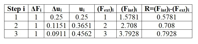
It is evident from the results that external and internal forces are NOT in equilibrium because Fexternal≠FInternal">Fexternal≠FInternalFexternal≠FInternal.
The following table summarizes the results for explicit analysis method.
Implicit scheme:
An implicit analysis is the same as the explicit analysis, except that at the end of each step Newton-Raphson iterations are used to enforce equilibrium before moving to the next step.
Basically, an incremental force is applied to advance the solution forward at the beginning of a step. However, internal forces and external forces will not be in equilibrium unless the
stiffness is linear for the given step.
Hence, in order to achieve equilibrium, corrections must be made to the displacement.
This is accomplished by using Newton-Raphson iterations to minimize the residual, R=FInternal-Fexternal">R=FInternal−FexternalR=FInternal-Fexternal
Expanding the residual as a Taylor series about the current displacement uj">ujuj gives
Rj+1=Rj(uj)+dR(uj)duδuj+1+...=Rj+k(uj)δuj+1+...">Rj+1=Rj(uj)+dR(uj)duδuj+1+...=Rj+k(uj)δuj+1+...Rj+1=Rj(uj)+dR(uj)duδuj+1+...=Rj+k(uj)δuj+1+...
By neglecting higher order terms in the series, setting Rj+1=0">Rj+1=0Rj+1=0 and solving for δuj+1">δuj+1δuj+1 the following correction is obtained
δuj+1=−[k(uj)]−1⋅Rj">δuj+1=−[k(uj)]−1⋅Rjδuj+1=−[k(uj)]−1⋅Rj
Here, the iteration variable is j and it may take several iterations for the norm of the residual, R, to be reduced below the chosen tolerance criteria of 0.01.
The implicit analysis proceeds as follows
Step-1̲">Step−1––––––––––Step-1̲
u0=0.0,⇒k(u0)=4,ΔF=1,Δu1=ΔFk(u0)=0.25,u1=u0+Δu1=0.25">u0=0.0,⇒k(u0)=4,ΔF=1,Δu1=ΔFk(u0)=0.25,u1=u0+Δu1=0.25u0=0.0,⇒k(u0)=4,ΔF=1,Δu1=ΔFk(u0)=0.25,u1=u0+Δu1=0.25
Checking the residual,
Fexternal=ΔF=1">Fexternal=ΔF=1Fexternal=ΔF=1
FInternal=u13+9u12+4u1=1.578">FInternal=u31+9u21+4u1=1.578FInternal=u13+9u12+4u1=1.578
R(0)=FInternal-Fexternal=0.578">R(0)=FInternal−Fexternal=0.578R(0)=FInternal-Fexternal=0.578
R(0)>10−2⇒">R(0)>10−2⇒R(0)>10−2⇒Newton-Raphson iterations are necessary.
Calculate the correction to u1=u1(0)">u1=u(0)1u1=u1(0)
δu(1)=−[k(u1(0))]−1⋅R(0)=-(8.6875)-1⋅0.578=-0.0665">δu(1)=−[k(u(0)1)]−1⋅R(0)=−(8.6875)−1⋅0.578=−0.0665δu(1)=−[k(u1(0))]−1⋅R(0)=-(8.6875)-1⋅0.578=-0.0665
⇒">⇒⇒The updated value of u1(1)=u1(0)+δu(1)=0.25-0.0665=0.1835">u(1)1=u(0)1+δu(1)=0.25−0.0665=0.1835u1(1)=u1(0)+δu(1)=0.25-0.0665=0.1835
Checking the residual again,
Fexternal=ΔF=1">Fexternal=ΔF=1Fexternal=ΔF=1
FInternal=(u1(1))3+9(u1(1))2+4u1(1)=1.0432">FInternal=(u(1)1)3+9(u(1)1)2+4u(1)1=1.0432FInternal=(u1(1))3+9(u1(1))2+4u1(1)=1.0432
R(1)=FInternal-Fexternal=0.0432">R(1)=FInternal−Fexternal=0.0432R(1)=FInternal-Fexternal=0.0432
R(1)>10−2⇒">R(1)>10−2⇒R(1)>10−2⇒Newton-Raphson iterations are necessary
Calculate the new total correction to u1=u1(0)">u1=u(0)1u1=u1(0)
δu(2)=δu(1)−[k(u1(1))]−1⋅R(1)=-0.0665-(7.404)-1⋅0.0432=-0.0723">δu(2)=δu(1)−[k(u(1)1)]−1⋅R(1)=−0.0665−(7.404)−1⋅0.0432=−0.0723δu(2)=δu(1)−[k(u1(1))]−1⋅R(1)=-0.0665-(7.404)-1⋅0.0432=-0.0723
The updated value of u1(2)=u1(0)+δu(2)=0.25-0.0723=0.1777">u(2)1=u(0)1+δu(2)=0.25−0.0723=0.1777u1(2)=u1(0)+δu(2)=0.25-0.0723=0.1777
Checking the residual again,
Fexternal=ΔF=1">Fexternal=ΔF=1Fexternal=ΔF=1
FInternal=(u1(2))3+9(u1(2))2+4u1(2)=1.0006">FInternal=(u(2)1)3+9(u(2)1)2+4u(2)1=1.0006FInternal=(u1(2))3+9(u1(2))2+4u1(2)=1.0006
R(2)=FInternal-Fexternal=0.0006">R(2)=FInternal−Fexternal=0.0006R(2)=FInternal-Fexternal=0.0006
R(2)<10−2⇒">R(2)<10−2⇒R(2)<10−2⇒Newton-Raphson iterations are not necessary
Therefore, the final value is u1=u1(2)=0.1777">u1=u(2)1=0.1777u1=u1(2)=0.1777
Step-2̲">Step−2––––––––––Step-2̲
u1=0.1777,⇒k(u1)=7.2933,ΔF=1,Δu2=ΔFk(u1)=0.1371,u2=u1+Δu2=0.3148">u1=0.1777,⇒k(u1)=7.2933,ΔF=1,Δu2=ΔFk(u1)=0.1371,u2=u1+Δu2=0.3148u1=0.1777,⇒k(u1)=7.2933,ΔF=1,Δu2=ΔFk(u1)=0.1371,u2=u1+Δu2=0.3148
Checking the residual,
Fexternal=ΔF+ΔF=2">Fexternal=ΔF+ΔF=2Fexternal=ΔF+ΔF=2
FInternal=u23+9u22+4u2=2.1822">FInternal=u32+9u22+4u2=2.1822FInternal=u23+9u22+4u2=2.1822
R(0)=FInternal-Fexternal=0.1822">R(0)=FInternal−Fexternal=0.1822R(0)=FInternal-Fexternal=0.1822
R(0)>10−2⇒">R(0)>10−2⇒R(0)>10−2⇒Newton-Raphson iterations are necessary.
Calculate the correction to u1=u1(0)">u1=u(0)1u1=u1(0)
δu(1)=−[k(u2(0))]−1⋅R(0)=-(9.9637)-1⋅0.1822=-0.0182">δu(1)=−[k(u(0)2)]−1⋅R(0)=−(9.9637)−1⋅0.1822=−0.0182δu(1)=−[k(u2(0))]−1⋅R(0)=-(9.9637)-1⋅0.1822=-0.0182
⇒">⇒⇒The updated value of u2(1)=u2(0)+δu(1)=0.3148-0.0182=0.2966">u(1)2=u(0)2+δu(1)=0.3148−0.0182=0.2966u2(1)=u2(0)+δu(1)=0.3148-0.0182=0.2966
Checking the residual again,
Fexternal=ΔF+ΔF=2">Fexternal=ΔF+ΔF=2Fexternal=ΔF+ΔF=2
FInternal=(u2(1))3+9(u2(1))2+4u2(1)=2.0042">FInternal=(u(1)2)3+9(u(1)2)2+4u(1)2=2.0042FInternal=(u2(1))3+9(u2(1))2+4u2(1)=2.0042
R(1)=FInternal-Fexternal=0.0042">R(1)=FInternal−Fexternal=0.0042R(1)=FInternal-Fexternal=0.0042
R(1)<10−2⇒">R(1)<10−2⇒R(1)<10−2⇒Newton-Raphson iterations are not necessary
Therefore, the final value is u2=u2(1)=0.2966">u2=u(1)2=0.2966u2=u2(1)=0.2966
Step-3̲">Step−3––––––––––Step-3̲
u2=0.2966,⇒k(u2)=9.6027,ΔF=1,Δu3=ΔFk(u2)=0.1041,u3=u2+Δu3=0.4007">u2=0.2966,⇒k(u2)=9.6027,ΔF=1,Δu3=ΔFk(u2)=0.1041,u3=u2+Δu3=0.4007u2=0.2966,⇒k(u2)=9.6027,ΔF=1,Δu3=ΔFk(u2)=0.1041,u3=u2+Δu3=0.4007
Checking the residual,
Fexternal=ΔF+ΔF+ΔF=3">Fexternal=ΔF+ΔF+ΔF=3Fexternal=ΔF+ΔF+ΔF=3
FInternal=u33+9u32+4u3=3.1121">FInternal=u33+9u23+4u3=3.1121FInternal=u33+9u32+4u3=3.1121
R(0)=FInternal-Fexternal=0.1121">R(0)=FInternal−Fexternal=0.1121R(0)=FInternal-Fexternal=0.1121
R(0)>10−2⇒">R(0)>10−2⇒R(0)>10−2⇒Newton-Raphson iterations are necessary.
Calculate the correction to u2=u2(0)">u2=u(0)2u2=u2(0)
δu(2)=−[k(u3(0))]−1⋅R(0)=-(11.6942)-1⋅0.1121=-0.00958">δu(2)=−[k(u(0)3)]−1⋅R(0)=−(11.6942)−1⋅0.1121=−0.00958δu(2)=−[k(u3(0))]−1⋅R(0)=-(11.6942)-1⋅0.1121=-0.00958
⇒">⇒⇒The updated value of u3(1)=u3(0)+δu(2)=0.4007-0.00958=0.3911">u(1)3=u(0)3+δu(2)=0.4007−0.00958=0.3911u3(1)=u3(0)+δu(2)=0.4007-0.00958=0.3911
Checking the residual again,
Fexternal=ΔF+ΔF+ΔF=3">Fexternal=ΔF+ΔF+ΔF=3Fexternal=ΔF+ΔF+ΔF=3
FInternal=(u3(1))3+9(u3(1))2+4u3(1)=3.0008">FInternal=(u(1)3)3+9(u(1)3)2+4u(1)3=3.0008FInternal=(u3(1))3+9(u3(1))2+4u3(1)=3.0008
R(1)=FInternal-Fexternal=0.0008">R(1)=FInternal−Fexternal=0.0008R(1)=FInternal-Fexternal=0.0008
R(1)<10−2⇒">R(1)<10−2⇒R(1)<10−2⇒Newton-Raphson iterations are not necessary
Therefore, the final value is u3=u3(2)=0.3911">u3=u(2)3=0.3911u3=u3(2)=0.3911
The results of the implicit analysis are summarized in the following table.
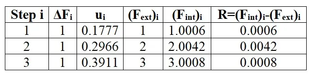
It is evident from the table that the external forces and internal forces are coming into equilibrium.
Inference:
A plot of the results is shown in below figure.
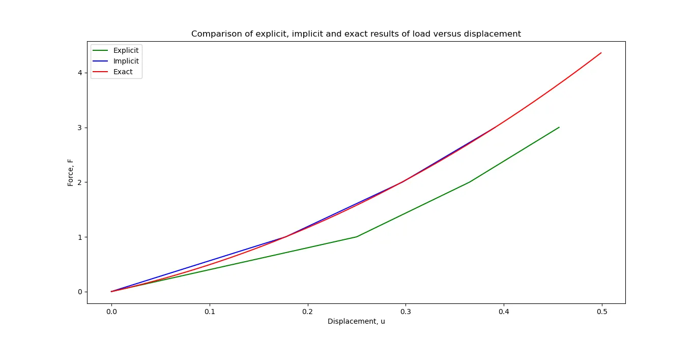
It is evident from the plot that the explicit analysis drifts from the exact solution.
The drift from the exact solution illustrates the lack of equilibrium between the internal and external forces. To correct for this problem an implicit analysis is required.
The Newton-Raphson iterations correct the incremental steps so that they land on the exact solution according to the specified tolerance. Excellent agreement is achieved with just 3 increments and in each step only two Newton-Raphson iterations are required.
Discussion:
As discussed, we can use both implicit and explicit solvers to solve the same type of problems. The only difference is in approach to time increment.
The implicit analysis allows you to select how big the time increment should be. This increment will take some time to compute since it has to iterate for global equilibrium first. But we can make it reasonably big for our analysis.
Explicit time increments calculate really fast because they do not iterate for global equilibrium, but the time increment there is not the user’s choice. Solver simply assumes an acceptable time increment and goes with it.
The speed of computing is exactly the difference between implicit and explicit. Of course, the size of explicit step depends on our model and computing times depends on the system hardware.