Week - 2 - Explicit and Implicit Analysis

Aim - To solve given equation with both Implicit and Explicit method and compare the obtained solution with exact solution to learn which of the two methods have better accuracy.

Implicit vs Explicit Analysis

Explicit Analysis – It is an incremental procedure which tends to update Stiffness matrix at the end of each increment and uses it for the next load increment/step. In case of Explicit method smaller incremental loads are applied to maintain accuracy as the solution would drift apart from exact solution if increments are larger.

Implicit Analysis – It is the same as Explicit Analysis with addition of a Newton Raphson iteration after every load increment to enforce equilibrium between applied force and internal force. Implicit analysis tends to be more accurate when compared to Explicit Analysis although computation cost is higher but at the same time could handle more complex loadings and deliver accurate results.

Given,

`f(u)= u^3+9u^2+4u`

Therefore `k(u)= 〖3u〗^2+18u+4`

Explicit Method

Step – 1

Considering displacement as 0

`u_o=0

k(u_o)=3(〖0)〗^2+18(0)+4=4`

`∆F=1`(Incrementing external force by value of 1)

`∆u_1=∆F/(k(u_o))=1/4=0.25

u_1=u_0+∆u_1=0+0.25=0.25`

Step - 2

`u_1=0.25

k(u_1)=3(〖0.25)〗^2+18(0.25)+4=8.6875`

`∆F=1`(Incrementing external force by value of 1)

`∆u_2=∆F/(k(u_1))=1/8.6875=0.1151

u_2=u_1+∆u_2=0.25+0.1151=0.3651`

Step -3

`u_2=0.3651

k(u_2)=3(〖0.3651)〗^2+18(0.3651)+4=10.9716`

`∆F=1`(Incrementing external force by value of 1)

`∆u_3=∆F/(k(u_2))=1/10.9716=0.0911

u_3=u_2+∆u_3=0.3651+0.0911=0.4562`

From the above 3 steps following results are obtained.

`F_ext=∆F+∆F+∆F=3

f_int=u_3^3+9u_3^2+4u_3

f_int=〖(0.4562)〗^3+9〖(0.4562)〗^2+4(0.4562)

f_int=3.7928`

It is evident from the above values that internal and external forces are not in equilibrium.

Step i	`∆F_i`	`∆u_i`	`u_i`	`(F_ext )_i`	`(f_int )_i`	`f_int-F_ext=R`
1	1	0.25	0.25	1	1.5781	0.5781
2	1	0.1151	0.3651	2	2.7087	0.7087
3	1	0.0911	0.4562	3	3.7928	0.7928

Implicit Method

Step – 1

`u_o=0

k(u_o)=3(〖0)〗^2+18(0)+4=4`

`∆F=1`(Incrementing external force by value of 1)

`∆u_1=∆F/(k(u_o))=1/4=0.25

u_1=u_0+∆u_1=0+0.25=0.25`

Check the Residual,

`F_ext=∆F=1

f_int=u_1^3+9u_1^2+4u_1= 〖0.25〗^3+9*〖0.25〗^2+4*0.25=1.5781

R^((0) )=f_int-F_ext=1.5781-1=0.5781`

`∥R^((0) )∥>〖10〗^(-2)`, Newton-Raphson iteration is necessary.

Calculate the correction to `u_1=u_1^((0) )`

`δu^((1))=-〖[k(u_1^((0) ))]〗^(-1) R^((0))

δu^((1))=-〖[3(〖0.25)〗^2+18(0.25)+4]〗^(-1)*0.5781

δu^((1))=-1/8.6875*0.5781= -0.0665`

The updated value of `u_1^((1) )=u_1^((0) )+δu^((1) )=0.25+(-0.0665)=0.1835`

Check the Residual again,

`F_ext=∆F=1

`f_int=〖〖(u〗_1^((1)))〗^3+9〖u_1^((1))〗^2+4u_1^((1))= 〖0.1835〗^3+9*〖0.1835〗^2+4*0.1835=1.0432

R^((1) )=f_int-F_ext=1.0432-1=0.0432

∥R^((1) )∥>〖10〗^(-2)`, Another Newton-Raphson iteration is necessary.

Calculate the correction to `u_1=u_1^((1) )`

`δu^((2))=δu^((1))-〖[k(u_1^((1) ))]〗^(-1) R^((1))

δu^((2) )=-0.0665-〖[3(〖0.1835)〗^2+18(0.1835)+4]〗^(-1)*0.0432

δu^((2) )= -0.072335`

The updated value of `u_1^((2) )=u_1^((0) )+δu^((2) )=0.25+(-0.072335)=0.177665`

Check the Residual again,

`F_ext=∆F=1

f_int=〖〖(u〗_1^((2)))〗^3+9〖u_1^((2))〗^2+4u_1^((2))= 〖0.177665〗^3+9*〖0.177665〗^2+4*0.177665=1.000354

R^((2) )=f_int-F_ext=1.000354-1=0.000354

∥R^((2) )∥<〖10〗^(-2)`,no further iteration is required.

Therefore, the final value is `〖u_1=u〗_1^((2) )=0.177665`

Step – 2

`k(u_1)=3(〖0.177665)〗^2+18(0.177665)+4=7.292671

∆F=1

∆u_2=∆F/(k(u_1))=1/7.292671=0.137124

u_2=u_1+∆u_2=0.177665+0.137124=0.314789`

Check the Residual,

`F_ext=2

f_int=〖u_2〗^3+9〖u_2〗^2+4u_2=〖0.314789〗^3+9*〖0.314789〗^2+4*0.314789=2.182181

R^((0) )=f_int-F_ext=2.182181-2=0.182181

∥R^((0) )∥>〖10〗^(-2)`, Newton-Raphson iteration is necessary.

Calculate the correction to `u_2=u_2^((0) )`

`δu^((1))=-〖[k(u_2^((0) ))]〗^(-1) R^((0))

δu^((1))=-〖[3(〖0.314789)〗^2+18(0.314789)+4]〗^(-1)*0.182181

δu^((1))=-1/9.963478*0.182181= -0.018285`

.The updated value of `u_2^((1) )=u_2^((0) )+δu^((1) )=0.314789+(-0.018285)=0.296504`

Check the Residual again,

`F_ext=2

f_int=〖〖(u〗_2^((1)))〗^3+9〖u_2^((1))〗^2+4u_2^((1))= 〖0.296504〗^3+9*〖0.296504〗^2+4*0.296504=2.003316

R^((1) )=f_int-F_ext=2.003316-2=0.003316

∥R^((1) )∥<〖10〗^(-2)`,no further iteration is required.

Therefore, the final value is `〖u_2=u〗_2^((1) )=0.296504`

Step – 3

`k(u_2)=3(〖0.296504)〗^2+18(0.296504)+4=9.600818`

`∆F=1`(Incrementing external force by value of 1)

`∆u_3=∆F/(k(u_2))=1/9.600818=0.104158

u_3=u_2+∆u_3=0.296504+0.104158=0.400662`

Check the Residual,

`F_ext=3

f_int=〖u_3〗^3+9〖u_3〗^2+4u_3=〖0.400662〗^3+9*〖0.400662〗^2+4*0.400662=3.111736

R^((0) )=f_int-F_ext=3.111736-3=0.111736

∥R^((0) )∥>〖10〗^(-2)`, Newton-Raphson iteration is necessary.

Calculate the correction to `u_3=u_3^((0) )`

`δu^((1))=-〖[k(u_3^((0) ))]〗^(-1) R^((0))

δu^((1))=-〖[3(〖0.400662)〗^2+18(0.400662)+4]〗^(-1)*0.111736

δu^((1))=-1/11.6935*0.111736= -0.009555`

The updated value of `u_3^((1) )=u_3^((0) )+δu^((1) )=0.400662+(-0.009555)=0.391107`

Check the Residual again,

`F_ext=3`

`f_int=〖〖(u〗_3^((1)))〗^3+9〖u_3^((1))〗^2+4u_3^((1))= 〖0.391107〗^3+9*〖0.391107〗^2+4*0.391107=3.00093

R^((1) )=f_int-F_ext=3.00093-3=0.00093

∥R^((1) )∥<〖10〗^(-2)`, no further iteration is required.

Therefore, the final value is `〖u_3=u〗_3^((1) )=0.391107`

Summary table for Implicit Method

`u_i`

Step i	`∆F_i`	`(F_ext )_i`	`(f_int )_i`	`f_int-F_ext=R`
1	1	0.177665	1	1.000354	0.000354
2	1	0.296504	2	2.003316	0.003316
3	1	0.391107	3	3.00093	0.00093

Calculation of Exact Values

`f(u)= u^3+9u^2+4u

If f(u)= u^3+9u^2+4u=1

u=0.177617

If f(u)= u^3+9u^2+4u=2

u=0.296159

If f(u)= u^3+9u^2+4u=3

u=0.391026`

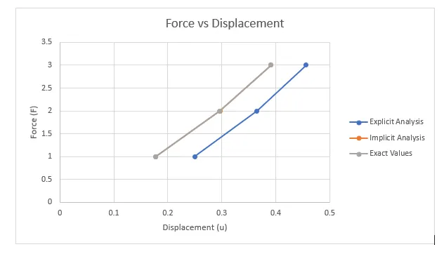
Data points of Exact Analysis and Implicit Analysis are very similar and hence graph shows same trend line for both data points.

Conclusion – From the above solution and graph it is evident that values obtained from Explicit Analysis drift apart from exact solution whereas values obtained from Implicit Analysis is very close to exact solution. That shows by using Newton Raphson iterative method equilibrium between Internal and external force is maintained.