Week - 2 - Explicit and Implicit Analysis

                                                      Explicit and Implicit Analysis

Aim:

As demonstrated in the example, "F(u) = u3+9u2+4u" using this equation to solve using both Explicit and Implicit analysis Methods ( have a tolerence of 0.001).

The Problem

Consider the case of a simple bar in tension and suppose that the force in the bar is a nonlinear function of the displacement

f(u) = u³+9u²+4u ----------------------------------------------------------(1)

From (1) it follows that the stiffness of the bar is k(u)

k(u) = df/du =3u²+18u+4--------------------------------------------. (2)

Explicit Analysis

Clearly it is possible to plot a graph of force, f, versus displacement, u, by using equation (1) . However, if the nonlinear force versus displacement relationship is not known, but the stiffness is known, it is possible to construct the graph of force versus displacement numerically.

One method is to use an incremental explicit load control scheme. This is illustrated next. For this example, three equal load increments (or steps) of ∆F = 1 unit each are used to load the tension bar.

The variables used are u for displacement, f for internal force in the bar, F for external force applied to the bar and k for stiffness.

Incremental displacements or incremental externally applied forces are represented as ∆u or ∆F, respectively. Use is made of the relationship ∆F = k∆u.

The analysis proceeds as follows:

Step 1

u0 = 0.0, ⇒ k(u0) =(3*0²)+(18*0)+4=4, ∆F = 1, ∆u1 = ∆F/k(u0) = 1/4, u1 = u0 + ∆u1 = 0+0.25=0.25

Step 2

⇒ k(u1) =(3*0.25²)+( 18*0.25)+4 =8.6875 , ∆F = 1, ∆u2 = ∆F/k(u1) = 1/8.6875=0.1151079136690, u2 = u1 + ∆u2 = 0.25+0.1151=0.3651

Step 3

⇒ k(u2) = (3*(0.3651)²) +( 18*0.3651) +4=10.97169403, ∆F = 1, ∆u3 = ∆F/k(u2) = 1/10.9716 = 0.09114, u3 = u2+∆u3 =0.3651+0.09114=0.4562436280729 ≈ 0.4562

Finally, from the three steps the following results are obtained.

F_ext = ∆F + ∆F + ∆F = 3.0

For u=u1=0.25, f_int = u³+9u²+4u = (0.25³) +( 9*0.25²) +(4*0.25) =1.578125 ≈ 1.5781

For u=u1=0.3651, f_int = u³+9u²+4u = (0.3651³) +( 9*0.3651²) + (4*0.3651) =2.67570709 ≈ 2.6757

For u=u1=0.4652, f_int = u³+9u²+4u = (0.4562³) +( 9*0.4562²) +(4*0.4562) =3.792809592328 ≈ 3.7928

It is evident from the results that external and internal forces are NOT in equilibrium because

F_ext ≠ F_int. Thus table 1 summarizes the main results for the explicit analysis.

                                   Table 1: Summary of explicit analysis results

Step i	∆Fi	∆ui	ui	(Fext)i	(fint)i	fint- Fext = R
1	1.0	0.2500	0.25	1.0	1.5781	0.5781
2	1.0	0.1151	0.3651	2.0	2.6757	0.6757
3	1.0	0.09114	0.4562	3.0	3.7928	0.7928

Implicit Analysis

An implicit analysis is the same as the explicit analysis, except that at the end of each step Newton-Raphson iterations are used to enforce equilibrium before moving to the next step. Basically, an incremental force is applied to advance the solution forward at the beginning of a step. However, internal forces and external forces will not be in equilibrium unless the stiffness is linear for the given step. Hence, in order to achieve equilibrium, corrections must be made to the displacement. This is accomplished by using Newton-Raphson iterations to minimize the residual, R(u) = f_int − F_ext. Expanding the residual as a Taylor series about the current displacement u j gives

                               R ^j+1 = R^j (u^j ) + (dR/du)(u^j) δu^j+4 + ... = R ^j + k(u^j )δu^j+1 + …………………….. (3)

By neglecting higher order terms in the series, setting Rj+1 = 0 and solving for δuj+1 the following correction is obtained

                                      δu^j+1 = −[k(u^j)]⁻¹R ^j …………………………………………………………………………….. (4)

Notice that the iteration variable is j and it may take several iterations for the norm of the residual, kRk, to be reduced below the chosen tolerance criteria (for the example below a tolerance of 10⁻³ is chosen). The implicit analysis proceeds as follows (results are approximate, they are more precise if done in a computer to machine precision.

Step 1

 u0 = 0.0, ⇒ k(u0) =(3*0²)+(18*0)+4=4 , ∆F = 1, ∆u1 = ∆F/k(u0) = 1/4, u1 = u0 + ∆u1 = 0.25

Check the residual,

F_ext = ∆F = 1, f_int = (0.25³) +( 9*0.25²) +(4*0.25) =1.578125 ≈ 1.5781,

R⁽⁰⁾ = f_int − F_ext = 1-1.5481=0.5781, R⁽⁰⁾ > 10⁻³ ⇒ Newton-Raphson iterations are necessary.

Calculate the correction to u1 = u (0)1 δu(1) = −[k(u(0))]⁻¹R(0) = -[((3*0.25²)+(18*0.25)+4)^-1 ]*(1.578)= −0.0665323741007=-0.06653 ⇒ The updated value of u (1) 1 = u (0) 1 + δu(1) = 0.25+ (−0.6652) = 0.1834676258992=0.1835

Check the residual again R¹,

Fext = ∆F = 1, fint = (0.1835³) +( 9*0.1835²) +(4*0.1835) ≈ 1.0432,

R⁽¹⁾ = f_int − F_ext = 1-1.0432=0. 0432, R ⁽⁰⁾ > 10⁻³ ⇒ Newton-Raphson iterations are necessary.

Calculate the correction to u1 = u1(1) δu(1) = −[k(u1(1))]⁻¹R(1) =(-0.6653)-(8.6875)^-1*(0.432) = -0.0714 ⇒ The updated value of u1 (1) = u1(2) + δu(2) = 0.25+ (−0.0714) = 0.1786

Check the residual again R2,

Fext = ∆F = 1, fint = (0.1786³) +( 9*0. 1786²) +(4*0. 1786) ≈ 1.0071,

R(2) = fint − Fext = 1-1.0071=0. 0071, R (2) > 10⁻³ ⇒ Newton-Raphson iterations are necessary.

Calculate the correction to u1 = u1(1) δu(1) = −[k(u1(1))]⁻¹R(1) =(-0.714)-(8.6875^-1)*(0.0071) =-0.07221 - ⇒ The updated value of u1 (1) = u1(2) + δu(2) = 0.25+ (−0.07221) = 0.1777

Check the residual again R3

Fext = ∆F = 1, fint = (0.1777³) +( 9*0. 1777²) +(4*0. 1777) ≈ 1.0006068,

R(2) = fint − Fext = 1.0006068-1=0. 0006068, R (3) < 10⁻³

Therefore, the final value is u1 = u (2) 1 = 0.1777.

Step 2

k(u1) =3u²+18u+4 = (3*0.1777²) + (18*0.1777) + 4 =7.29333, ∆F = 1, ∆u2 = ∆F/k(u1) = 1/7.29333=0.1371115, u2 = u1 + ∆u2 =0.314811 ≈ 0.3148

Check the residual, Fext = ∆F = 1, fint = u³+9u²+4u = 2.18228

R(0) = fint − Fext =2.18228-2= 0.18228

 R⁽⁰⁾ > 10⁻³ ⇒ Newton-Raphson iterations are necessary.

Calculate the correction to u₂ = u₂⁽⁰⁾

δu⁽¹⁾ = −[k(u₂⁽⁰⁾)]⁻¹R⁽⁰⁾ = −2.70874⁻¹ (0.18228) = −0.06729. ⇒ The updated value of u₂ ⁽¹⁾ = u₂⁽⁰⁾ + δu⁽¹⁾ = 0.314811   + (−0.06729) = 0.24751

Check the residual again,

Fext = 1, Fext = ∆F = 1, fint = u³+9u²+4u = 1.5565

R⁽¹⁾ = fint − Fext =1.5565-1 =0.5565

R⁽¹⁾ > 10⁻³ ⇒ another Newton-Raphson iteration is necessary.

Calculate the new total correction to u₂ = u₂⁽⁰⁾

δu⁽²⁾ = δu⁽¹⁾ − [k(u₂⁽¹⁾)]⁻¹R⁽¹⁾ = −0.06729 − (2.70874⁻¹)* 0.5565 = −0.27273.

The updated value of u₂⁽²⁾ = u₂⁽⁰⁾ + δu⁽²⁾ = 0.3651 + (−0.27273) = 0.042081.

Check the residual,

F_ext = 1, f_int = u³+9u²+4u =0.44722  

R⁽²⁾ = f_int − F_ext = 0.44722 – 1=-0.5527

 R(2) < 10⁻³ ⇒ no further iterations are necessary.

Therefore, the final value is u2 = u (2) 2 = 0.042081

 

Step 3

it is completed similar to steps 1 and 2, the final values of u3 = 0.3911. The results of the implicit analysis are summarized in Table 2. It is evident from the table that the external forces and internal forces are coming into equilibrium.

                                         Table 2: Summary of implicit analysis results

Step i	∆Fi	∆ui	ui	(Fext)i	(fint)i	fint- Fext = R
1	1	0.25	0.1777	1	1.0006068	0.0006068
2	1	0.1347	0.042081	2	0.44722	-0.5527
3	1	0.0.1041	0.3911	3	3.0008	0.0008

Plot of results

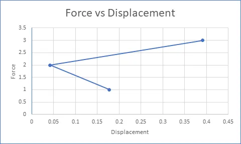
A plot of the results is shown in Figure (a). It is evident from the plot that the explicit analysis drifts from the exact solution. If 20 increments are used the explicit analysis more closely follows the exact solution as shown in Figure (b). However, even with more increments the explicit analysis still drifts from the exact solution. The drift from the exact solution illustrates the lack of equilibrium between the internal and external forces. To correct for this problem an implicit analysis is required. The results for the implicit analysis are shown in Figure(b).

The Newton-Raphson iterations correct the incremental steps so that they land on the exact solution according to the specified tolerance. Excellent agreement is achieved with just 3 increments and in each step only two Newton-Raphson iterations are required.

Figure (a)

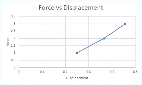
Figure (b)

Discussion

In practice a more sophisticated convergence criteria may be necessary when solving complex structures with many degrees of freedom. However, for this example problem minimization of the norm of the residual is a sufficient criterion. It is important to note how the initial increment due to the incremental load advances the solution forward. Then if an implicit analysis is employed, Newton-Raphson iterations are used to make corrections to the displacement in order to achieve equilibrium. Once satisfactory equilibrium is achieved, a new load increment is applied to advance the solution and the process is repeated. Note that an exact expression for force versus displacement is not always known.

Conclusion

 A nonlinear analysis is illustrated using an incremental explicit and implicit procedure. The results are plotted for comparison. It is evident from the results that the explicit analysis drifts from the true solution. To overcome this problem an implicit analysis is used, which includes Newton-Raphson iterations to enforce equilibrium between internal and external forces. The techniques demonstrated are for a load control scheme.

Thus the equation F(u) = u³+9u²+4u is solved using both Explicit and Implicit Methods with a tolerence of 0.001.