Week - 2 - Explicit and Implicit Analysis
Aim
The aim of this challenge is to compare the characteristics and quality of the results obtained by the two most used solution schemes for FEA Analyses (Explicit and implicit methods). By plotting the results obtained with both methods, a visual tool to identify the accuracy of the solutions will be obtained.
Calculations
`f(u) = u^3+9u^2+4u`
`k(u)=frac{df}{du}=3u^2+18u+4`
Explicit Method
For step 1
`u0=0`
`k(u0)=3(0)^2+18(0)+4=4`
`Delta F = 1`
`Delta u1= frac {Delta F}{k(u0)} = frac{1}{4}=0.25`
`u1=u0+Deltau1=0+0.25=0.25`
`Fext=1`
`F"int"= 0.25^3+9(0.25)^2+4*0.25= 1.578125`
`R=F"int"-Fext= 1.578125-1= 0.578125`
For step 2
`u1=0.25`
`k(u1)=3(0.25)^2+18(0.25)+4=8.6875`
`Delta F = 1`
`Delta u2= frac {Delta F}{k(u1)} = frac{1}{8.6875}=0.1151`
`u2=u1+Deltau2=0.25+0.1151=0.3651`
`Fext=2`
`F"int"= 0.3651^3+9(0.3651)^2+4*0.3651= 2.7088`
`R=F"int"-Fext=2.7088-2=0.7088`
For step 3
`u2=0.3651`
`k(u3)=3(0.3651)^2+18(0.3651)+4=10.9719`
`Delta F = 1`
`Delta u3= frac {Delta F}{k(u3)} = frac{1}{10.9719}=0.0911`
`u3=u2+Deltau3=0.3615+0.0911=0.45625`
`Fext=3`
`F"int"=0.45625^3+9(0.45625)^2+4*0.45625=3.79345`
`R=F"int"-Fext=3.79345-3=0.79345`
Implicit Method
Tolerance for iterations = 10^-3
For step 1
`u0=0`
`k(u0)=3(0)^2+18(0)+4=4`
`Delta F = 1`
`Delta u1= frac {Delta F}{k(u0)} = frac{1}{4}=0.25`
`u1=u0+Deltau1=0+0.25=0.25`
`Fext=1`
`F"int"=0.25^3+9*(0.25)^2+4*(0.25)=1.5781`
`R=F"int"-Fext=1.5781-1=0.5781`
`abs(R)>10^-3`
So a new Newton Rhapson iteration is required
Calculate correction to u1
`deltau_1^1=-[k(u_1^0)]^-1*R^0=-8.6875^-1*(0.5781)=-0.0665`
The update the value of
`u_1^1 = u_1^0 + delta u_1^1 = 0.25 + (-0.0665)=0.1834`
For iteration 2
`u_1^1 =0.1834`
`f"int" = 0.1834^3+9*(0.1834)^2+4*(0.1834)=1.0429`
`Fext=1`
`R=F"int"-Fext=0.0428`
`abs(R)>10^-3`
So a new Newton-Rhapson iteration is required
Calculate correction to u1
`deltau_1^2=deltau_1^1-[k(u_1^1)]^-1*R^1=-0.0665-7.4031^-1*(0.0428)=-0.0723`
The update the value of
`u_1^2 = u_1^0 + delta u_1^2 = 0.25 + (-0.0723)=0.17766`
For iteration 3
`u_1^2 =0.17766`
`f"int" = 0.17766^3+9*(0.17766)^2+4*(0.17766)=1.0003`
`Fext=1`
`R=F"int"-Fext=0.0003`
`abs(R)<10^-3`
So no iterations are required and the values for the first step are:
`u1 =0.17766`
`f"int_1" = 1.0003`
For step 2
`u1=0.17766`
`k(u1)=3(0.17766)^2+18(0.17766)+4=7.2926`
`Delta F = 1`
`Delta u2= frac {Delta F}{k(u1)} = frac{1}{7.2926}=0.1371`
`u2=u1+Deltau2=0.17766+0.1371=0.3148`
`Fext=2`
`F"int"=0.3148^3+9*(0.3148)^2+4*(0.3148)=2.1822`
`R=F"int"-Fext=2.1822-2=0.1822`
`abs(R)>10^-3`
So a new Newton-Rhapson iteration is required
Calculate correction to u2
`deltau_2^1=-[k(u_2^0)]^-1*R^0=-9.9634^-1*(0.1822)=-0.0183`
The update the value of
`u_2^1 = u_2^0 + delta u_2^1 = 0.3148+ (-0.0183)=0.2965`
For iteration 2
`u_2^1 =0.2965`
`f"int" = 0.2965^3+9*(0.2965)^2+4*(0.2965)=2.0033`
`Fext=2`
`R=F"int"-Fext=0.0033`
`abs(R)>10^-3`
So a new Newton-Rhapson iteration is required
Calculate correction to u2
`deltau_2^2=deltau_2^1-[k(u_1^1)]^-1*R^1=-0.0183-9.9634^-1*(0.0033)=-0.01863`
The update the value of
`u_2^2 = u_2^0 + delta u_2^2 = 0.3148 + (-0.01863)=0.2962`
For iteration 3
`u_2^2 =0.2962`
`f"int" = 0.2962^3+9*(0.2962)^2+4*(0.2962)=2.000001`
`Fext=2`
`R=F"int"-Fext=0.000001`
`abs(R)<10^-3`
So no iterations are required and the values for the first step are:
`u2 =0.2962`
`f"int"_2 = 2.000001`
For step 3
`u2=0.2962`
`k(u2)=3(0.2962)^2+18(0.2962)+4=9.5940`
`Delta F = 1`
`Delta u3= frac {Delta F}{k(u1)} = frac{1}{9.5940}=0.1042`
`u2=u1+Deltau2=0.2962+0.1042=0.4004`
`Fext=3`
`F"int"=0.4004^3+9*(0.4004)^2+4*(0.4004)=3.1086`
`R=F"int"-Fext=3.1086-3=0.1086`
`abs(R)>10^-3`
So a new Newton Rhapson iteration is required
Calculate correction to u3
`deltau_3^1=-[k(u_3^0)]^-1*R^0=-11.6880^-1*(0.1086)=-0.0093`
The update the value of
`u_3^1 = u_2^0 + delta u_2^1 = 0.4004+ (-0.0093)=0.3911`
For iteration 2
`u_3^1 =0.3911`
`f"int" = 0.3911^3+9*(0.3911)^2+4*(0.3911)=3.0009`
`Fext=3`
`R=F"int"-Fext=0.0009`
`abs(R)<10^-3`
So no iterations are required and the values for the first step are:
`u3 =0.3911`
`f"int"_3 = 3.0009`
Results
With the values calculated for both explicit and implicit schemes, we get the following table
| Step i | Delta F_i | u_i | (F_Ext)_i | (f_"int")_ i | f_"int"-F_ext =R |
| 0 | 0 | 0 | 0 | 0 | 0 |
| 1 | 1 | 0.25 | 1 | 1.578125 | 0.578125 |
| 2 | 1 | 0.3651079 | 2 | 2.708836 | 0.70883602 |
| 3 | 1 | 0.4562502 | 3 | 3.793454 | 0.79345417 |
Table 1. Explicit Solution
| Step i | Delta F_i | u_i | (F_Ext)_i | (f_"int")_ i | f_"int"-F_ext =R |
| 0 | 0 | 0 | 0 | 0 | 0 |
| 1 | 1 | 0.177661 | 1 | 1.00032 | 0.000320254 |
| 2 | 1 | 0.296159 | 2 | 2.000001 | 1.18085E-06 |
| 3 | 1 | 0.391102 | 3 | 3.000879 | 0.000879337 |
Table 2. Implicit Solution
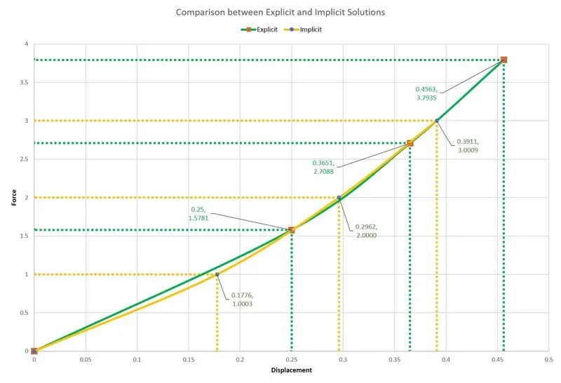
And the corresponding graphs look like this:
Conclusion
The graphs look similar in their trajectory, but the results obtained by the implicit method give much more acurrate results.
From the tables 1 and 2, it can be seen that the value for R in the explicit scheme for each time step is quite large in comparison to the implicit one. This tells us that the force applied to the beam member is not quite in equilibrium in the explicit method, thus the results may not be that accurate. A good recommendation would be to increase the steps by decreasing the delta Force to capture the curve better. The explicit scheme reduces the amount of calculations required (because there are no Newton-Rhapson iterations), but the accuracy is not that good with so few steps.
In the implicit scheme, the correction factor calculated in internal iterations reduces the residual, making every step equilibrated in the external and internal forces. A possible constraint for the implicit method is that the residual does not converge to a value less than the tolerance selected, because if this happens, Newton-Rhapson iterations can diverge and make impossible the solution.