Week - 2 - Explicit and Implicit Analysis

Explicit and Implicit Analyses

Aim: The aim of this report is to highlight the differences in explicit and implicit time discretization approaches when it comes to solving non-linear problems.

Introduction: When solving time-dependent problems in FEA, it is necessary to discretize the whole time span of the solution into smaller intervals. This is done in order to study the response of the structure or part under load at different time intervals or load levels. There are two broad approaches to time discretization, namely implicit and explicit, that are used depending on the type of problem being solved and the numerical stability and accuracy required. These methods have been described in further detail in the next section of the report. Apart from the theoretical framework, the report will resort to a sample problem of a bar in tension having a certain displacement function. The results of the outcome from both approaches will be discussed and relevant inferences will be drawn.

Theoretical Framework:

• Explicit Method: In the explicit method, the variable under consideration is computed in terms of known quantities from the previous time step.

  Example: Consider the force-displacement problem of F(u) = du/dt...................................(i)

  Here F is the force as a function of the displacement u.

  The explicit method will give the solution as:

u(n+1) = u(n) + `delta`t . F(u(n))............................(ii)

The basic equation to be solved is

m(d2u/dt2) + ku = F...............................................(iii)

Using the known values of u(n), m and k are computed for the current time-step. Acceleration is computed using these values of m and k and then velocity and displacement are computed at `delta`t using the acceleration.

a = M`-1`(F-ku)..............................(iv)

v(`delta`t) = v(0) +at......................(v)

u(`delta`t) = u(0) + v`delta`t + 0.5a`delta`t2..............(vi)

The stability of explicit simulations depends on the size of the time-step. The time-step needs to be lower than the threshold given by Courant-Friedrick-Levy's condition:

`delta`t < L.`square root`(`rho`(1-2`nu`)/(2`mu`(1-`nu`)).......(vii)

This is the time taken by a sound wave to travel through the length (L) of an element having material density `rho`, Poissons ratio `nu`, and viscosity `mu`.Explicit methods find more use in dynamic problems.

• Implicit Method: In the implicit method the displacement or any other concerned variable is computed in terms of variables from both the current and the previous time step. For the problem given by equation (i),

The implicit method will compute the displacement at time-step (n+1) as:

u(n+1) = u(n) + `delta`t . F(u(n+1))......................(vii)

Since the unknown parameters (at the current time-step) occur at both the left and right-hand sides of the equation, it is said to be implicit in nature. Solutions are computed in an iterative nature. Here, m and k are computed at time `delta`t and the rest of the steps follows as in equations (iv), (v), and (vi).

In static problems, at every time step, the solution must be in equilibrium i.e. the external force (F) must be equal to the internal force (f) = k(u).du and the residual force R = F-f = 0. For dynamic problems, the external force F = m.a, where (m) is the mass of the body and (a) is the acceleration of the body. To achieve this equilibrium, certain corrections are made to the displacement (to linearise the stiffness matrix).

Implicit simulations are unconditionally stable and the time-step is usually larger than in the explicit method but is limited by the required accuracy of the results as well as the computation cost/time.

Implicit methods are more commonly used to solve static and quasi-static problems.

Problem: To understand the difference between the implicit and explicit methods in a more practical manner, consider the following non-linear static problem of a bar being loaded in tension with an external force F.

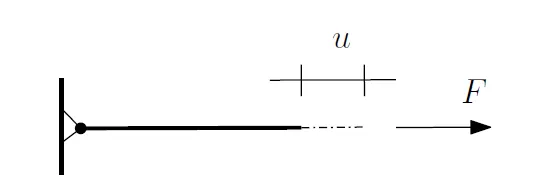
Fig 1: Bar under tension

The non-linear force-displacement relation is as follows:

f(u) = u`cube`+ 9u`square`+ 4u.................................(ix)

The stiffness of the bar is given by:

k(u) = df/du = 3u`square`+ 18u + 4.............................(x)

The problem is solved by the incremental load step method for both the implicit and explicit approaches i.e. at each step the externally applied force `delta`F = 1 unit. Also the initial displacement u_0 = 0 units.

• Explicit Method: The explicit method algorithm follows as shown below:

incremental force`delta`F = 1

initial displacement u_0 = 0

incremental displacement `delta`u_(i+1) = `delta`F/k(u_i)

displacement at step (i+1) u_(i+1) = u_i + `delta`u_(i+1)

External Force F_ext = `sum``delta`F

Internal Force f_int = f(u_i)

Residual unbalanced force R = f_int - F_ext

Using the above logic, a MATLAB code was written to solve the problem for three load steps or a total load of 3units. A snippet of the code is shown below:

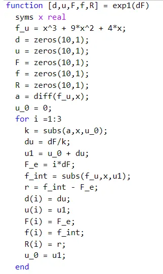
The output from the above code is shown in the table below:

Step	`delta`F	u_i	F_ext	f_int	R = f_int - F_ext
1	1	0.2500	1	1.5781	0.5781
2	1	0.3651	2	2.7088	0.7088
3	1	0.4563	3	3.7935	0.7935

Table 1: Explicit method results

• Implicit method: The implicit method algorithm is as follows:

incremental force`delta`F = 1

initial displacement u_0 = 0

incremental displacement `delta`u_(i+1) = `delta`F/k(u_i)

displacement at step (i+1) u_(i+1) = u_i + `delta`u_(i+1)

External Force F_ext = `sum``delta`F

Internal Force f_int = f(u_i)

Residual unbalanced force R = f_int - F_ext

If `mod`R > 10^(-2) i.e. if the residual forces exceed a specified tolerance, then some corrections are made to the displacment using the Newton-Raphson method:

du(1) = du_0 - [R_0/k(u_i_0)]

u_i_1 = u_i_0 + du(1)

f_int(1) = k(u_i_1)

R_1 = f_int(1) - F_ext

The iterations above are repeated until the residual drops below the specified tolerance.

Using the above logic, a MATLAB code was written, a snippet of which is as shown below:

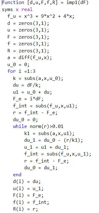
The results from the solution are shown below:

Step	`delta`F	u_i	F_ext	f_int	R = f_int - F_ext
1	1	0.1785	1	1.0066	0.0066
2	1	0.2697	2	2.0051	0.0051
3	1	0.3914	3	3.0040	0.0040

Table 2: Implicit Method results

Discussion: From Table 1, it can be seen that the displacement and hence the internal force in the case of the explicit method is quite high leading to high unbalanced forces in the system. This will show up as some form of motion or deformation in the model in a simulation and the results won't be an accurate representation of the actual physical world phenomenon.

By correcting the displacement at each iteration in the implicit method, the internal forces are reduced and the unbalanced forces are far lower and the overall system is in equilibrium. The tolerance value in this problem is very high (0.01). For narrower tolerances, the internal and external forces will almost be the same.

The Force displacement plot of the two methods further highlights the gap in the results:

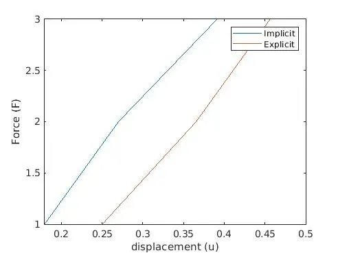
Fig 2: Force-displacement plot

Conclusion: To solve the given static non-linear problem, the implicit method gives a more accurate solution as in static problems, the summation of all forces should be zero or the system must be in equilibrium. This highlights the efficacy of the implicit method when solving static problems.