Week - 2 - Explicit and Implicit Analysis

Aim: To solve the given equation f (u) = u³+9u²+4u by using the explicit and implicit methods constraining the residual tolerance as 10^-2.

Procedure: The given equation is having the non-linear static relation between the forces (F) in the function of displacement (u). In the given equation both Explicit and Implicit Method is solved by using incremental load scheme.

Explicit Method:

In this method, in the given equation consists of force and displacement relationship. By differentiating the force w.r.t displacement, stiffness equation is obtained. By using the initial element formation at each incremental load step we are solving for all variable in respective element. By using the previous the elemental variables and increasing the load incremental as inputs and solving the next element.

For the given equation f (u) = u³+9u²+4u is defines as non-linear relation of force and displacement,

Now, differentiation the above force function with displacement, stiffness is obtained.

K (u) = d K(u) / d(u)

K (u) = 3u²+18u+4

For this problem we are considering the load incremental as ∆F = 1 for 3 load steps for the given bar,

The variables u for displacement, f for internal force, F for external force on bar and k for stiffness. Further incremental external load is represented as ∆F and incremental displacement as ∆U.

Step: 1

At Initial displacement u_o = 0, ∆F = 1 , following parameter are calculated as follows

K (u₀) = 4 , ∆u₁ = = 0.25 ,

Next displacement u₁ = u_{o +} ∆u₁ = 0.25

F_external = 1,

f_internal = f(u₁) = 1.5781

Step 2 : Initial inputs u₁ = 0.25, ∆F = 1

K (u₁) = 8.688 , ∆u₂ = = 0.1151

Next displacement u₂ = u_{1 +} ∆u₂ = 0.3651

F_external = 2,

f_internal = f(u₂) = 2.708

Step 3 : Initial inputs u₁ = 0.25, ∆F = 1

K (u₂) = 10.9717, ∆u₃ = = 0.0911

Next displacement u₃ = u_{2 +} ∆u₂ = 0.4562

F_external = 3,

f_internal = f(u₃) = 3.7928

From the above we can observe F_external is not equal to f_internal , the given equation is not in equilibrium

The Following output table.1 is summarized by using the explicit analysis,

Step i	∆F i	∆ui	Ui	finternal	Fexternal	Resultant
1	1	0.25	0.25	1.5781	1	0.5781
2	1	0.1151	0.3651	2.708	2	0.708
3	1	0.0911	0.4562	3.7928	3	0.7928

Implicit Method:

In this method, in the given equation consists of force and displacement relationship. By differentiating the force w.r.t displacement, stiffness equation is obtained but to get maintain the equilibrium before proceeding to next step after end of each step Newton-Raphson iteration are used to modulate the Residual tolerance. Basically, an incremental force is applied to advance the solution forward at the beginning of a step. However, internal forces and external forces will not be in equilibrium unless the stiffness is linear for the given step. Hence, in order to achieve equilibrium, corrections must be made to the displacement. This is accomplished by using Newton-Raphson iterations to minimize the residual, R (u) = fint − Fext. Expanding the residual as a Taylor series about the current displacement u_i.

R^j+1 = R^j (u^j) + δ u^j+1 + ….. = Rj + k(uj) δ u^j+1 + ……….

The following correction is obtained By neglecting higher order terms in the series, setting R^j+1= 0 and solving for

δu^j+1 = −[k(u^j)]^-1R^j

here the iteration is done is repeated for several times before proceeding the next load incremental step until residual R is reduced to given tolerance 0.01.

By using the initial element formation at each incremental load step we are solving for all variable in respective element. By using the previous the elemental variables and increasing the load incremental as inputs and solving the next element.

For the given equation f (u) = u³+9u²+4u is defines as non-linear relation of force and displacement,

Step: 1

At Initial displacement u_o = 0, ∆F = 1 , following parameter are calculated as follows

K (u₀) = 4 , ∆u₁ = = 0.25 ,

Next displacement u₁ = u_{o +} ∆u₁ = 0.25

F_external = 1,

f_internal = f(u₁) = 1.5781

R⁽⁰⁾ = f_internal - F_external = 0.578

R⁽⁰⁾ > 0.01, go to next iteration by using Newton-Raphson Method, calculate the updated displacement

δu ⁽¹⁾ = −[k(u₁⁽⁰⁾)]^-1R⁽⁰⁾

= -0.0665

u₁⁽¹⁾ = u_o ⁽⁰⁾+ δu⁽¹⁾ = 0.25-0.0665 = 0.1835 (Iteration 1)

F_external = 1,

f_internal = f(u₁) = 1.0432

R⁽¹⁾ = f_internal - F_external = 0.0432

R⁽²⁾ > 0.01, go to next iteration by using Newton-Raphson Method, calculate the updated displacement

δu ⁽²⁾ = δu ⁽¹⁾ −[k(u₁⁽¹⁾)]^-1R⁽¹⁾

= -0.0723

u₁⁽²⁾ = u_o ⁽¹⁾+ δu⁽²⁾ = 0.25-0.0723= 0.1777 (Iteration 2)

F_external = 1,

f_internal = f(u₁) = 1.0006

R⁽⁰⁾ = f_internal - F_external = 0.0006

R ⁽²⁾ < 0.01, go to next Load incremental step, final Value u₁ = u₁ ⁽²⁾ = 0.1777

Step: 2

At Initial displacement u₁ = 0.1777, ∆F = 1 , following parameter are calculated as follows

K (u₁) = 7.2933, ∆u₂ = = 0.1371,

Next displacement u₂ = u_{1 +} ∆u₂ = 0.3148

F_external = 2,

f_internal = f(u₁) = 2.1822

R ⁽⁰⁾ = F_external -f_internal= 0.1822

R ⁽⁰⁾ > 0.01, go to next iteration by using Newton-Raphson Method, calculate the updated displacement

δu ⁽¹⁾ = −[k(u₁⁽⁰⁾)]^-1R⁽⁰⁾

= -0.0182

U₂ ⁽¹⁾ = u₁ ⁽⁰⁾+ δu⁽¹⁾ = 0.3148-0.0182 = 0.2966 (Iteration 1)

F_external = 2,

f_internal = f(u₂) = 2.0042

R ⁽¹⁾ = f_internal - F_external = 0.0042

R ⁽²⁾ < 0.01, go to next Load incremental step, final Value u₂ = u₂⁽¹⁾ = 0.2966

Step: 3

At Initial displacement u₂ = 0.2966, ∆F = 1 , following parameter are calculated as follows

K (u₂) = 9.6027, ∆u₃ = = 0.1041,

Next displacement u₃ = u_{2 +} ∆u₃ = 0.4007

F_external = 3,

f_internal = f(u₃) = 3.1121

R ⁽⁰⁾ = f_internal - F_external = 0.1121

R ⁽⁰⁾ > 0.01, go to next iteration by using Newton-Raphson Method, calculate the updated displacement

δu ⁽²⁾ = −[k(u₂⁽¹⁾)]^-1R⁽⁰⁾

= -0.00958

U₃⁽¹⁾ = u₃ ⁽⁰⁾+ δu⁽²⁾ = 0.4007-0.00958 = 0.3911 (Iteration 1)

F_external = 3,

f_internal = f(u₃) = 3.0008

R⁽¹⁾ = f_internal - F_external = 0.0008

R⁽¹⁾ < 0.01, terminate the iteration, final Value u₃ = u₃⁽¹⁾ = 0.3911

The Following output table.2 is summarized by using the implicit analysis,

Step i	∆F i	Ui	finternal	Fexternal	Resultant	No.of iterations
1	1	0.1777	1.0006	1	0.0006	2
2	1	0.2966	2.0042	2	0.0042	1
3	1	0.3911	3.0008	3	0.0008	1

Plot of Results

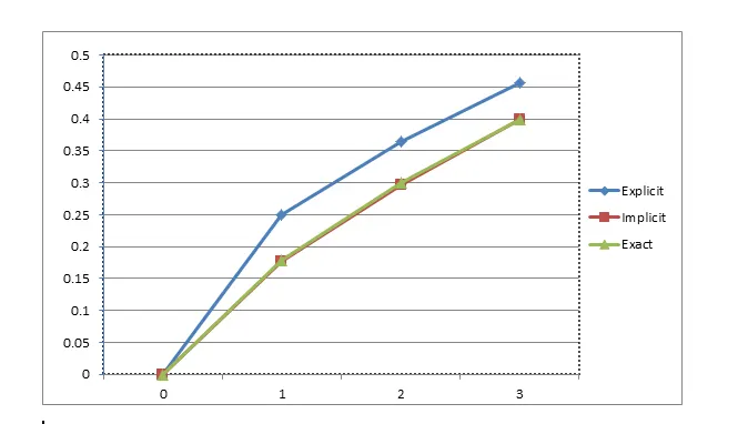
In the above figure.1 force is represented in abscissa and displacement in ordinate for implicit, explicit, exact solution respectively. If we observe the implicit and exact solution follows the same path but explicit is quite deviated from the exact solution, due to the iteration followed in the implicit to maintain the equilibrium condition. Further displacement obtained due to iteration is more in explicit analysis compare to other methodology, in implicit to maintain the global equilibrium of bar under external forces by constraining residual tolerance 0.01.

Conclusions:

1. Both the explicit and implicit methods are used to solve static and dynamic methods.
2. Implicit follows the procedure of iterations but explicit give direct solution. For this reason implicit converges towards the exact solution.
3. Direct solutions obtained in explicit but in implicit obtained by newton rapson methods.
4. In every step both the incremental load and stiffness matrix is updated.
5. Implicit method will consume more time than the explicit due to iterations.
6. Implicit is more accurate the explicit.
7. Implicit is unconditionally stable but explicit is condition stable, due to this in explicit the time increment is considered very small.
8. In implicit there is no mathematical time limit, but in explicit it depends upon the wave propagation, speed and characteristic length of element.
9. In implicit there the strain rates or velocity is very less than compare to explicit.