Week - 2 - Explicit and Implicit Analysis

OBJECTIVE:

To solve the given equation, F(u) = `u^3+9u^2+4u` using both Explicit and Implicit Methods have a tolerance of `10^-2`.

The explanation for the methods:

Implicit:

• When the problem is nonlinear, the solution is obtained in several steps and the solution for the current step is based on the solution from the previous step.
• For large models, inverting the matrix is highly expensive and will require advanced iterative solvers (over standard direct solvers).
• Sometimes, this is also known as the backward Euler. These solutions are unconditionally stable and facilitate larger time steps.
• Despite this advantage, the implicit methods can be extremely time-consuming when solving dynamic and nonlinear problems. The implicit method should be used when the events are much slower and the effects of strain rates are minimal.
• Once the growth of stress as a function of strain can be established, these can be analyzed using implicit methods. 3

Explicit:

• The explicit Method is a time-dependent method. It is used to solve Non-linear equation problems. Since there is a condition for the method to be stable, it is called a conditionally stable method.
• In this method the force and acceleration of the methods various rapidly within a short period of time. As compared to the implicit method here we don't need to solve inverse k matrix instead we solve inverse mass(m) matrix which will be a diagonal matrix.
• In most cases, the mass matrix is considered as “lumped” and thus a diagonal matrix. Inversion of a diagonal matrix is straightforward and includes inversion of the terms on the diagonal only.
• Once the accelerations are calculated at the nth step, the velocity at the n+1/2 step and displacement at the n+1 step are calculated accordingly. In these calculations, the scheme is not unconditionally stable and thus smaller time steps are required.

Problem and Explanation:

Given Equation:`F(u)=u^3 + 9u^2 +4u`

• The variables used are u for displacement, f for internal force in the bar, F for the external force applied to the bar, and k for stiffness. Incremental displacements or incremental externally applied forces are represented as `Delta`u or,`DeltaF`
  respectively. Use is made of the relationship ∆F = k∆u. The analysis proceeds as follows:

Solution based on Explicit Method:

Step1:

`u0 =0.0`

`k(u0)=3(u0)^2 +18(u0) +4`

=`3(0)^2 + 18(0)+4`

= 4

`DeltaF1 = 1 Rightarrow Deltau1 = ((DeltaF1)/(k(u0))) = 1/4`

`Deltau1 = 0.25`

`u1 = u0+Deltau1`

`u1 = 0.25`

Step 2:

`u1 = 0.25`

`k(u1) =3(u1)^2 + 18(u1) +4`

=`3(0.25)^2 +18(0.25)+4`

`k(u1) = 8.69`

`Delta F2 = 1, Rightarrow Deltau2 = (DeltaF2)/(k(u1)`

`Deltau2 =0.12`

`u2 = u1+Deltau2`

`u2 = 0.37`

Step 3:

`u2 =0.37`

`k(u2)=3(u2)^2+18(u2)+4`

`k(u1)=11.07`

`DeltaF3 =1, Rightarrow Deltau3 =(DeltaF3)/(k(u1)`

`Deltau3=0.09`

`u3 u2+Deltau3`

`u3=0.46`

From the above three-step, the following results are obtained.

`Fext = DeltaF1+DeltaF2+DeltaF3`

=`1+1+1=3`

`Fext = 3`

`FInt = (u3)^3+9(u3)^2+4(u3)`

=`(0.46)^3+9(0.46)^2+4(0.46)`

`FInt cong 3.85`

It is very clear from the result that external and internal force is not in equilibrium.

Tabulated Values:

Step	`DeltaFi`	`Deltaui`	`ui`	`(Fext)i`	`(FInt)i`	`R=FInt-Fext`
1	1	0.25	0.25	1	1.58	0.58
2	1	0.11	0.37	2	2.76	0.76
3	1	0.09	0.46	3	3.85	0.85

Solution based on Implicit Method:

Step1:

`DeltaF=1`

`k(u0)=3(u0)^2 +18(u0)+4`

`k(u0) = 3(0)+18(u0)+4`

`Deltau1 = (DeltaF)/(k(u0)) =1/4 =0.25`

`u1=u0+Deltau1=0+0.25=0.25`

`F(u1)=(u1)^3+9(u1)^2 +4(u1)`

`F(u1)=(0.25)^3+9(0.25)^2+4(0.25)=1.578`

`Fext = DeltaF = 1`

`R = F(u1)-Fext=1.578-1=0.578`

• Since`||R||>0.01`, Newton-Raphson iterations have to be done to obtain a correction factor to bring the R-value within the tolerance.

Correction Factor :`u1 = delu(1)1=-[k(u(0)1]^-1R^0`

`delu(1)^1=-[8.688]^-1 .0.578-=0.00665'`

Updated value of`u1=u(1)^1=u1+delu(1)^1=0.25+(-0.00665)=0.183`

`F(1)=((u(1)^1)^3+(9)u(1)^1)^2+4(u(1)^1))`

`F(1)=(0.183)^3+9(0.183)=1.039`

Residual,`R(1)=F(1)-Fext=1.039-1=0.039`

`||R||` is not within tolerance limit>We need to do correction Factor one more time

Correction factor for `u1=delu(2)^1=delu(1)^1-[k(u(1)^1]^(-1)R^(1)`

`k(u(1)^1)=3(0.183)^2+18(0.183)+4=7.394``R(1)=0.039`

`delu(2)^1=-0.0665-[7.394]^(-1).0.039=-0.0718`

Updated Value of u2 = `u^1+delu(2)^1=0.25+(-0.0718)=0.1782`

`F(2)=(0.1782)^3+9(0.1783)^2+4(0.1782)=1.004`

Residual,`R^2=F(2)-Fext=1.004-1=0.004`

Within tolerance Limit

Step 2:

`DeltaF=1`

`k(u1)=3(u1)^2+18(u1)+4=3(0.1782)^2+18(0.1782)+4=7.302`

`delu2=(delF)/(k(u1)) =(1/7.302)=0.137``u2=u1+delu2=0.178+0.137=0.315`

`F(u2)=(u2)^3+9(u2)^2+4u2=(0.315)^3+9(0.315)^2+4(0.315)=2.184`

`Fext=delF+delF=1+1=2`

`R=F(u2)-Fext=2.184-2=0.184`

Interation:

`k(u2)=9.967``R^0=0.184`

Correction Factor for`u2`is:

`deltau_2^1=-[k(u_2^0)]^-0R^0`

`deltau_2^1 = -[9.967]^-1 .0184=-0.0185`

Corrected`u2 :u2=u2+deltau_2^1=0.315+(-0.0185)=0.296`

`F^1=(u_2^1)^3+9(u_2^1)^2+4u_2^1`

`F1=0.296^3+9(0.296)^2+4(0.0296)=1.998`

Updated residual:`R^1=F^1-Fext=1.998-2=-0.002`

`||R||<0.01`,it has reached within the tolerance limit. so no need to further interation

Step 3:

`k(u2)=3(u2)^2+18(u2)+4=3(0.296)^2+18(0.296)+4=9.59`

`delu3=(delF)/(k(u2)) =1/9.59=0.104`

`u3=u2+du3=0.296+0.104=0.4`

`F(u3)=(u3)^3+9(u3)^2+4u3=0.4+9(0.4)^2+4(0.4)=3.104`

`Fext=delF+delF+delF=1+1+1=3`

`R=F(u3)-Fext=3.104-3=0.104`

Iteration:

`u3=0.4`

`k(u_3^0)=3(0.4)^2+18(0.4)+4=11.68`

`R_0=0.104`

`deltau_3^1=-[k(u_3^0)]^-0R^0`

`deltau_2^1=-[11.68]^-1. 0.104=-0.0089`

`u_3=u_3+deltau_3^1=0.4+(-0.0089)=0.3911`

`F^1=(u_3^1)^3+9(u_3^1)^2+4(u_3^1)`

`F^1=(0.3911)^3+9(0.3911)^2+4(0.3911)=3.0008`

`R^1=F^1-Fext=3.008-3=-0.0008`

`||R||<0.01`,it has reached within the tolerance limit.so no need to further iteration

Tabulated Values:

Step i	`ui`	Corrected`(ui)`	`DeltaF`	`Fext`	`FInt`	Corrected`FInt`	`R`
1	0.250	0.178	1	1	1.57	1	0.57
2	0.365	0.296	1	2	2.70	2	0.70
3	0.456	0.391	1	3	3.79	3	0.76

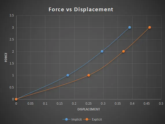
Diagramatic Representation:

Conclusion:

• Thus the given third-order polynomial equation under a tensile force is analytically solved both in the Implicit and Explicit method. Results are plotted in the graph and reported the same as shown above image.