Week 2 Bevel Gear Challenge

Objective :

To understand the concept of the Grid Dependency test and run the simulation on the bevel gear using three different mesh sizes i.e. 4mm, 5mm, and 6mm, and solving the simulation cases to evaluate Von-Mises stress, Equivalent elastic strain, and Total Deformation on the bevel gear using Ansys Workbench.

Theory on Grid Dependency Test :

• Grid Dependency Test is used to find out how the solution depends on the grid size by running the simulation with refined mesh i.e. finer the mesh, higher is the accuracy of the result but with additional cost on consumption time and consumption power.
• As solutions are interpolated at the nodes to get an approximate result, the higher the no. of nodes and elements higher is the computational time and power required to complete the simulation.
• With the help of the Grid Dependency Test, we can determine the optimal mesh size, where accurate results are obtained keeping in the mind the cost of time and power. The optimal mesh size obtained is neither too coarse nor fine and further refining the mesh would result in negligible percent change in the result but will increase the computational cost.

Procedure:

• Static Structural Analysis on Spur Gear is carried out in Ansys Workbench.
• Select Static Structural analysis from the Analysis System drop-down menu.
• Select the type of material required from the Engineering Data. In this case, Structural Steel is used.

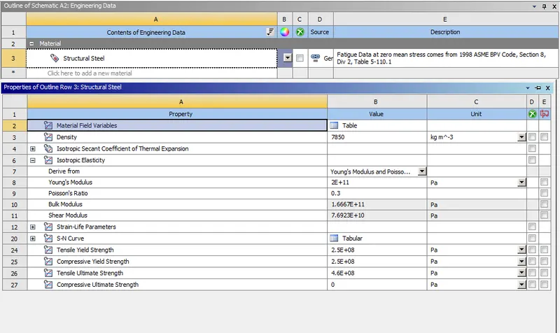
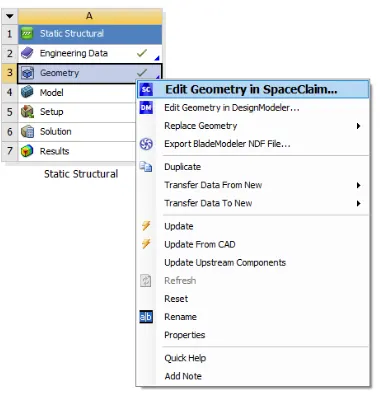
• Import the given geometry (Bevel Gear Model) and Open the model in SpaceClaim.

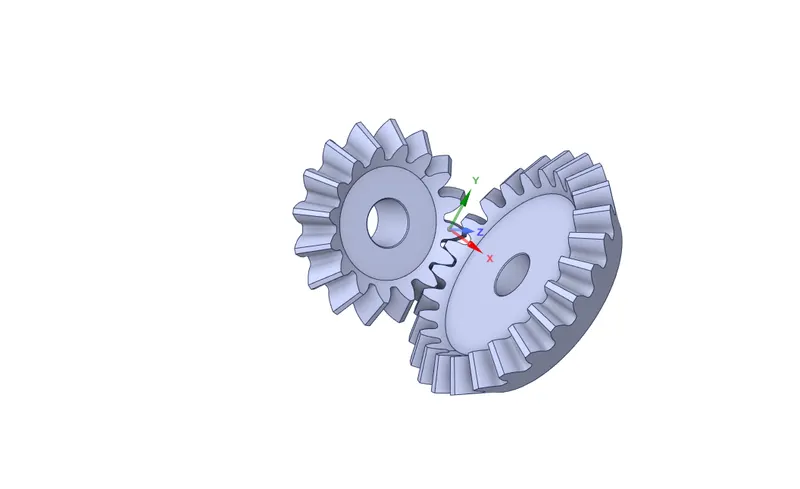
• After opening the model in SpaceClaim, edit the model by removing the unwanted extra surface which is not required for the simulation process by cutting down a circle with dia. 45mm for the big gear and another circle with dia. 25mm for the small gear.

BEFORE

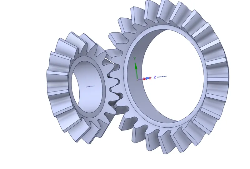
• Model after unnecessary surfaces are removed

• Open the model in Design Modeler
• Rename the Gears as Big and Small Gears and Assign the material.
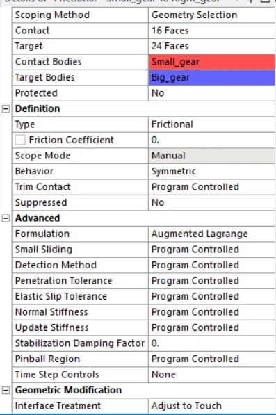
• Contacts are established between the small gear and the big gear.
• Contact Type is defined as Frictional.
• The mating surfaces of the Gears are selected as Contact and Target. The small gear is selected as Contact Body and the big gear is selected as Target body.
• Behaviour is defined as Symmetric.
• Formulation Type used in Augmented Lagrange.
• Interface Treatment is changed to Adjust to Touch.

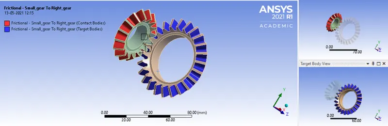
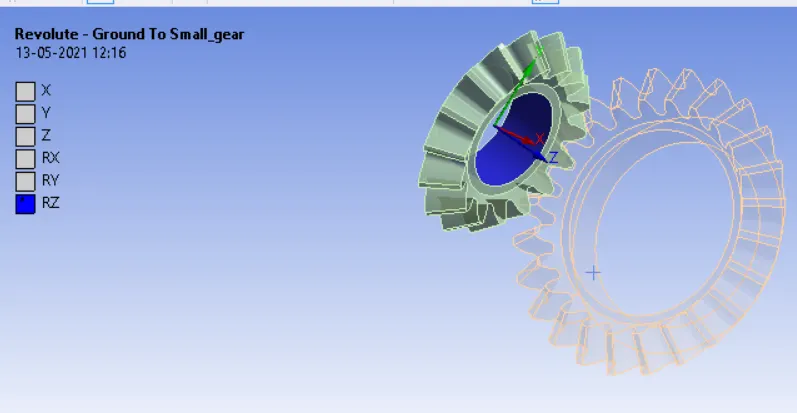
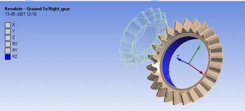
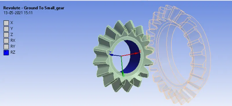
• After Creating Contacts between the gears, Revolute type Joints are assigned for both the gears having a Body – Ground Connection.

ANALYSIS SETTINGS :

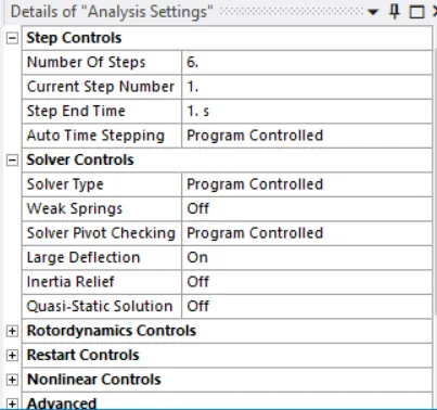
• The simulation runs for 6 Steps, So the no. of steps is set to 6.
• The 6 Steps that are created are selected and hence we get the Current Step Number as Multi-Step.
• Due to convergence issues, change the Auto Time Stepping to Program controlled.

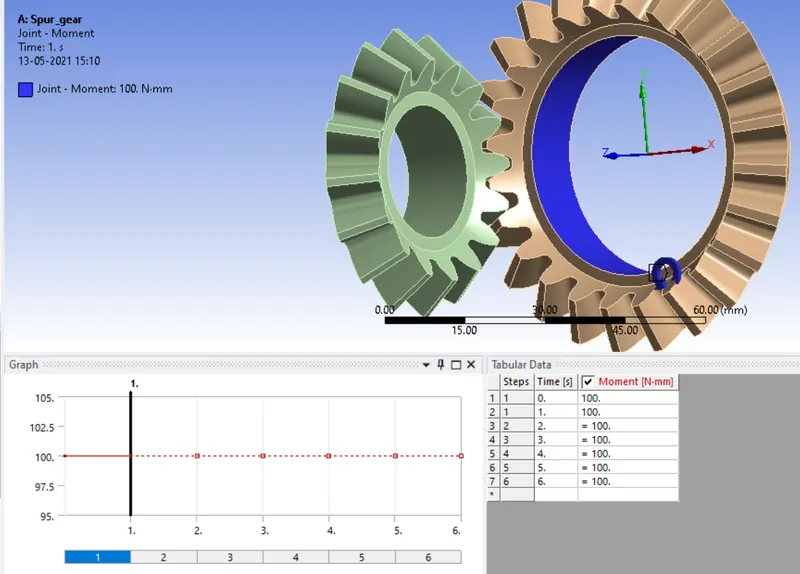
• After Setting up the Analysis Setting, Joint loads are given to the gears. Small Gear is given a Revolution Join Load for six-time steps and Large Gear is given a constant Moment Joint Load.

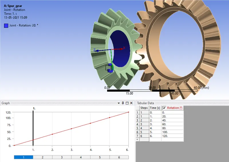
• Joint Revolution Load for Small Gear
• Make sure that the gears are rotating in opposite direction. If the gears are found to be rotating in the same direction, change the direction of rotation of either one of the gears by changing the Reference Coordinate System.

MESH :

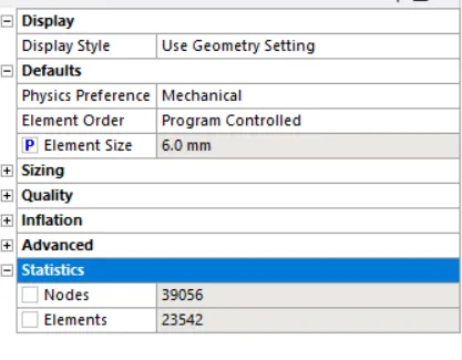
• After the Analysis Setup is done, Generate a Mesh using the default conditions. We can observe that the mesh generated is coarse and needs refinement as it will result in convergence issues.
• To prevent the mesh from being too coarse, we use mesh face sizing. Right-click in Mesh, select Insert and click on Sizing.
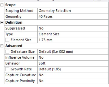
• Select the faces of the gear that come in contact. A Total of 40 faces is observed. Keep the face sizing element size as 1.75mm.

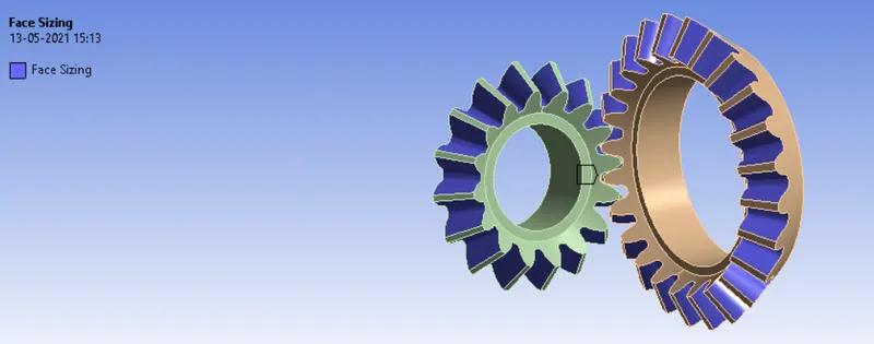
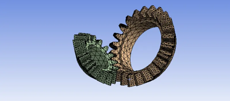
• The Mesh generated using Face Sizing is observed to be much better than the previously generated Mesh.

Parameterization:

• Now before solving for requested results, we have to give parameters to the Input as well as Output side.
• For Input parameters, we will give Mesh size and for Output parameters, we can give Minimum and maximum values for stress, strain, and deformation results.
• So we can select checkboxes given for input and output parameters as their locations as given below:

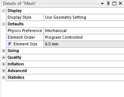
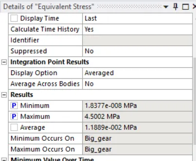
• After the creation of Parameters, solve the results and close the mechanical Module.
• We can see Parameter Set has been activated as given below:

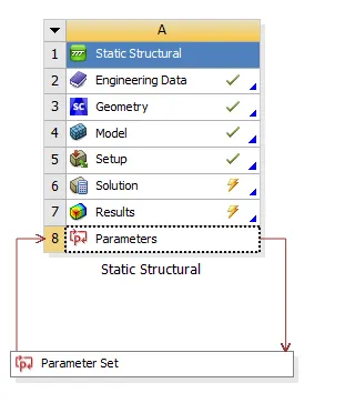
• By opening Parameter Set, we can see all Parameters in details as given below:

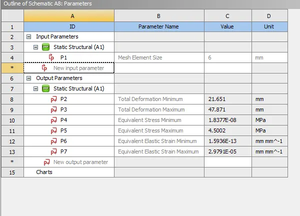
• In the above image, we can see the Input parameter as P1 and the Output parameters from P2 to P7
• We can also see the Design point we created as given below:

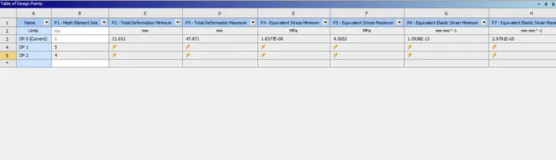
• Create new design points for 5 mm and 4 mm mesh and make sure that the “Retain” option is enabled.
• After giving all design points select “Update All Design Points” and get results for all design points.
• Results for updated design points will be as given below:

• So we can get all results very easily and fast by giving parameters as shown in the above image.

Results:

• By setting each Design Point as current, we can get results for each case as below:

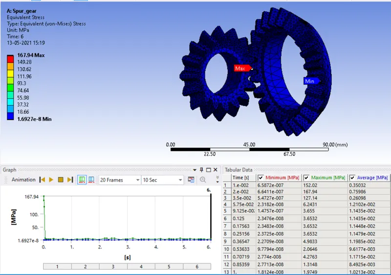
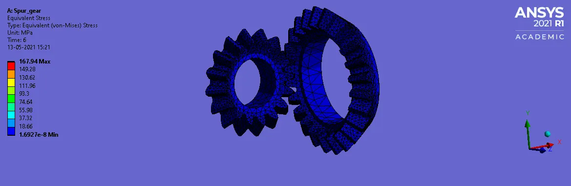
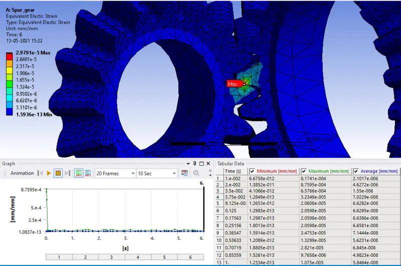
CASE_1: 6 mm

Stress Contours:

GIF:

Strain Contours:

GIF:

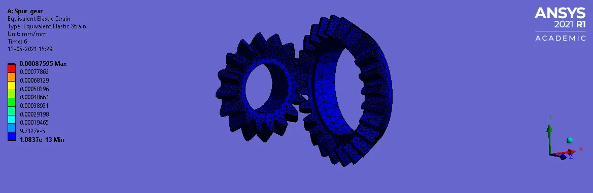
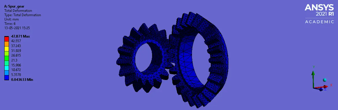
Deformation Contours:

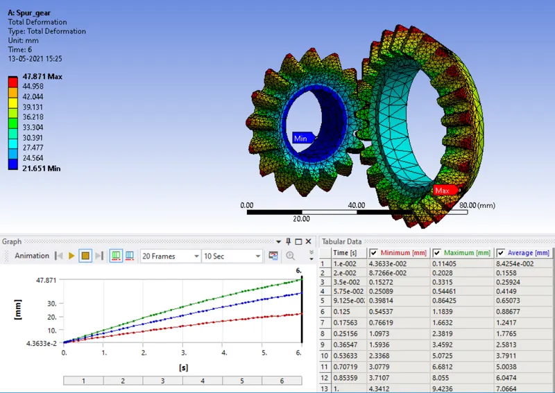
GIF:

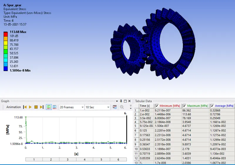
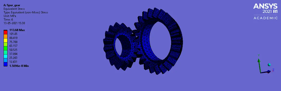
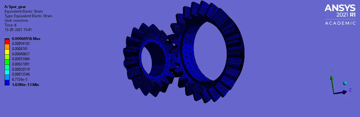
CASE_2: 5 mm

Stress Contours:

GIF:

Strain Contours:

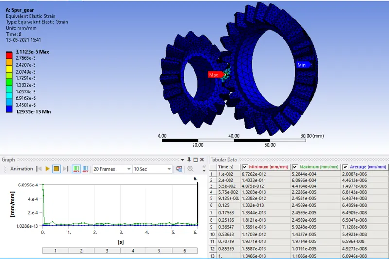
GIF:

Deformation Contours:

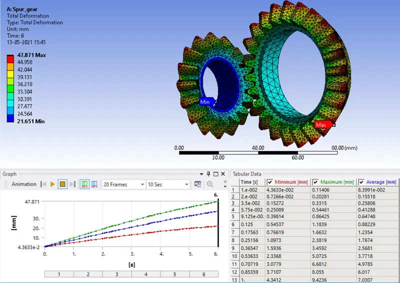
GIF:

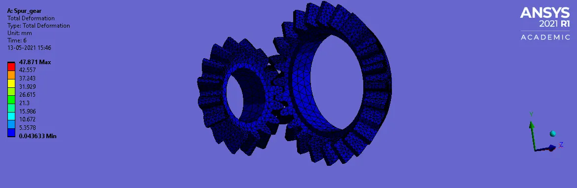
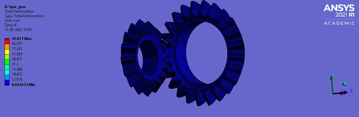
CASE_3: 4 mm

Stress Contours:

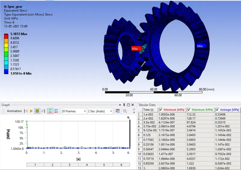
GIF:

Strain Contours:

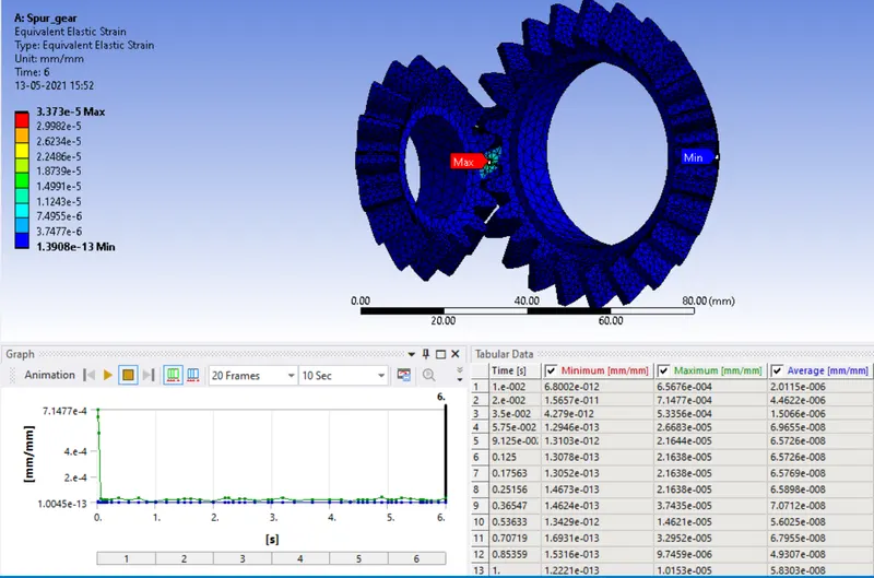
GIF:

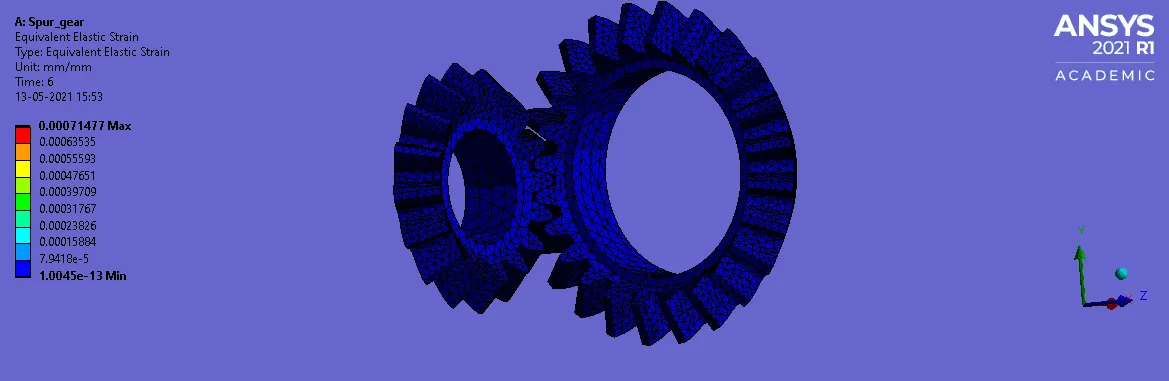
Deformation Contours:

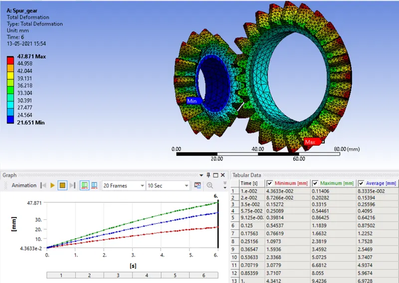
GIF:

Comparison:

Mesh Size	Min. Equivalent Stress ( MPa )	Max. Equivalent Stress ( MPa )	Min. Equivalent Strain	Max. Equivalent Strain	Min. Deformation ( mm )	Max. Deformation ( mm )
6mm	1.8377E-08	4.5002	1.5936E-13	2.9791E-05	21.651	47.871
5mm	1.5096E-08	4.7514	1.2935E-13	3.1123E-05	21.651	47.871
4mm	1.9597E-08	5.1855	1.3908E-13	3.373E-05	21.651	47.871

• From the above table, we can see that Case_2 and Case_3 are nearly similar and Case_1 values are lower in comparison.
• Also, we can see that maximum deformation occurs on Big Gear due to the moment.

For more comparative solution on-grid test we will see the Plot of Maximum Stress Vs Time for all three cases as given below:

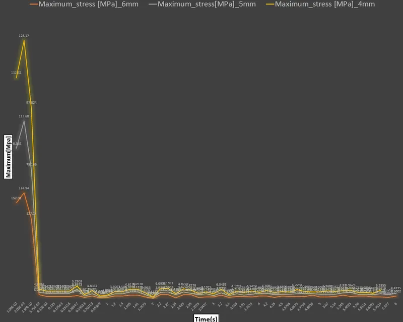
• Here we can see that the line plot of Case_2 is better than Case_1 and the plot of Case_3 is better than Case_2.
• In Case_3 there are more elements and nodes due to finer mesh compared to Case_1 and Case_2.
• So results are better calculated for Case_3 with the higher number of elements.

Conclusion:

• Grid Dependency test has been performed and From the above table and plot, we can conclude performing a grid dependency test on bevel gear by varying the global size of the mesh we achieve much better accuracy of the result. We can observe that as the mesh is refined from 6mm to 5mm and 5mm to 4mm we achieve better approximate of the result for equivalent elastic strain and equivalent stress, however, performing the simulation with further refining the mesh would result in a very close approximation of the result but with very negligible change in the result with an additional on the computational power and time.