Week 2 Air standard Cycle
OTTO CYCLE
The Otto cycle can be represented on a Pressure-Volume (PV) diagram, which helps visualize the changes in pressure and volume throughout the four stages of the cycle. Here's a description of the Otto cycle on a PV diagram:
Stage 1: Intake (Process 1-2): In this stage, the intake valve is open, and the piston moves downward, drawing in the air-fuel mixture. This process occurs at approximately constant pressure and is represented by a horizontal line on the PV diagram as the volume increases.
Stage 2: Compression (Process 2-3): Once the intake valve closes, the piston moves upward, compressing the air-fuel mixture. This process is adiabatic, meaning there is no heat transfer with the surroundings. As a result, both pressure and temperature increase significantly. On the PV diagram, this process is represented by a steep diagonal line as the volume decreases.
Stage 3: Power (Combustion) (Process 3-4): At the top of the compression stroke, the spark plug ignites the compressed air-fuel mixture, causing rapid combustion. The high-pressure gases push the piston downward, performing work on the piston. This process is also adiabatic and occurs at approximately constant volume on the PV diagram, resulting in a horizontal line as pressure decreases.
Stage 4: Exhaust (Process 4-1):Finally, the exhaust valve opens, and the piston moves upward again, pushing the burned gases out of the combustion chamber. This process occurs at approximately constant pressure as the volume increases, and it is represented by another horizontal line on the PV diagram.
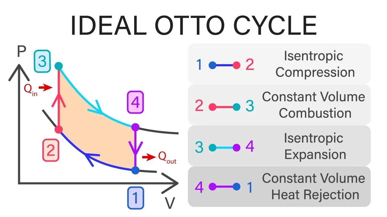
The completed cycle forms a closed loop on the PV diagram, representing one complete cycle of operation in the engine. The area enclosed by the loop represents the net work done by the engine during one cycle. The efficiency of the engine can be determined by comparing this work to the energy input from the fuel.
Code Procedure:
1) Define Basic engine parameters such as bore,stroke, connecting rod length, compression ratio.
2) Define initial stage parameters such as pressure, clearance & swept volume.
3) Code to identify state point paramters using Formula :
PV^gamma = k and PV/T =k
4) As we know, Volume will not be increasing linearly, we have to use formula to match the real cycle characteristics.
V/Vc = 1+ 0.5(cr-10)* [ R+1 -cos(angle) — (R² -sin²(angle)⁰.5]
5) Assign multiple values for crank angle(theta) in order to plot one complete cycle.
6) Use functions ,loops whenever necessary to reduce code.
7) Calculate Thermal efficiency and output its value.
7) Plot PV diagram with proper title,label,legend.
Python Code:
# OTTO CYCLE
import math
import matplotlib.pyplot as plt
def engine_kinematics(bore,stroke,c_rod,cr,start_crank,end_crank):
a = stroke/2 # crank pin radius
R = c_rod/a
sc = math.radians(start_crank)
ec = math.radians(end_crank)
num_values = 50
dtheta= (ec-sc)/(num_values-1)
V = []
for i in range(0,num_values):
theta = sc + i*dtheta
term1 = 0.5*(cr-1)
term2 = R + 1 - math.cos(theta)
term3 = pow(pow(R,2)-pow(math.sin(theta),2),0.5)
V.append((1 + term1*(term2-term3))*v_c)
return V
#Inputs
v0 = 0
p0 = 0
p1 = 101325
t1 = 500
gamma = 1.4
t3 = 2300
#Geometric parameters
bore = 0.1
stroke= 0.1
c_rod = 0.15
cr = 12
#Volume Computation
v_s = (math.pi/4)*pow(bore,2)*stroke
v_c = v_s/(cr-1)
v1 = v_c + v_s
#state point 2
v2 = v_c
p2 = p1*pow(v1,gamma)/pow(v2,gamma) #p2v2*gamma = p1v1*gamma
rhs = p1*v1/t1
t2 = p2*v2/rhs #p2v2/t2 = p1v1/t1
V_comp= engine_kinematics(bore,stroke,c_rod,cr,180,0)
constant = p2*pow(v2,gamma)
P_comp= []
for v in V_comp:
P_comp.append(constant/pow(v,gamma))
#state point 3
v3 = v2
p3 = rhs*t3/v3 # p3v3/t3 = p2v2/t2 and rhs is constant ratio
V_exp = engine_kinematics(bore,stroke,c_rod,cr,0,180)
constant = p3*pow(v3,gamma)
P_exp = []
for v in V_exp:
P_exp.append(constant/pow(v,gamma))
#state point 4
v4 = v1
p4 = p3*pow(v3,gamma)/pow(v4,gamma) #p4v4*gamma = p3v3*gamma
t4 = p4*v4/rhs #p4v4/t4 = p3v3/t3(rhs)
# Plots
plt.figure(1)
plt.plot([v0,v1],[p0,p1])
plt.plot(V_comp,P_comp,label='Isentropic compression')
plt.plot([v2,v3],[p2,p3],label='Constant volume Combustion')
plt.plot(V_exp,P_exp,label='Isentropic expansion')
plt.plot([v4,v1],[p4,p1],label='Constant volume heat rejection')
plt.xlabel('Volume')
plt.ylabel('Pressure')
plt.legend()
plt.savefig('Otto cycle PV diagram')
plt.show()
#thermal efficiency
eff=1-(1/pow(cr,(gamma-1)))
eff=str(eff*100)
print('Thermal Efficiency =' + eff + '%')
Results
1) PV diagram
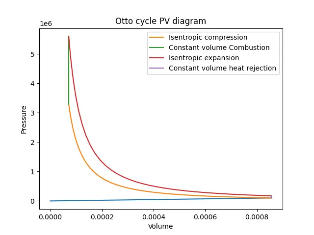
Inference : Our result exactly coincides with the PV cycle image ( given above) and properly explains all the 5 stages. The plot is also labeled and legend is added to explain the stages.
2) Thermal efficiency
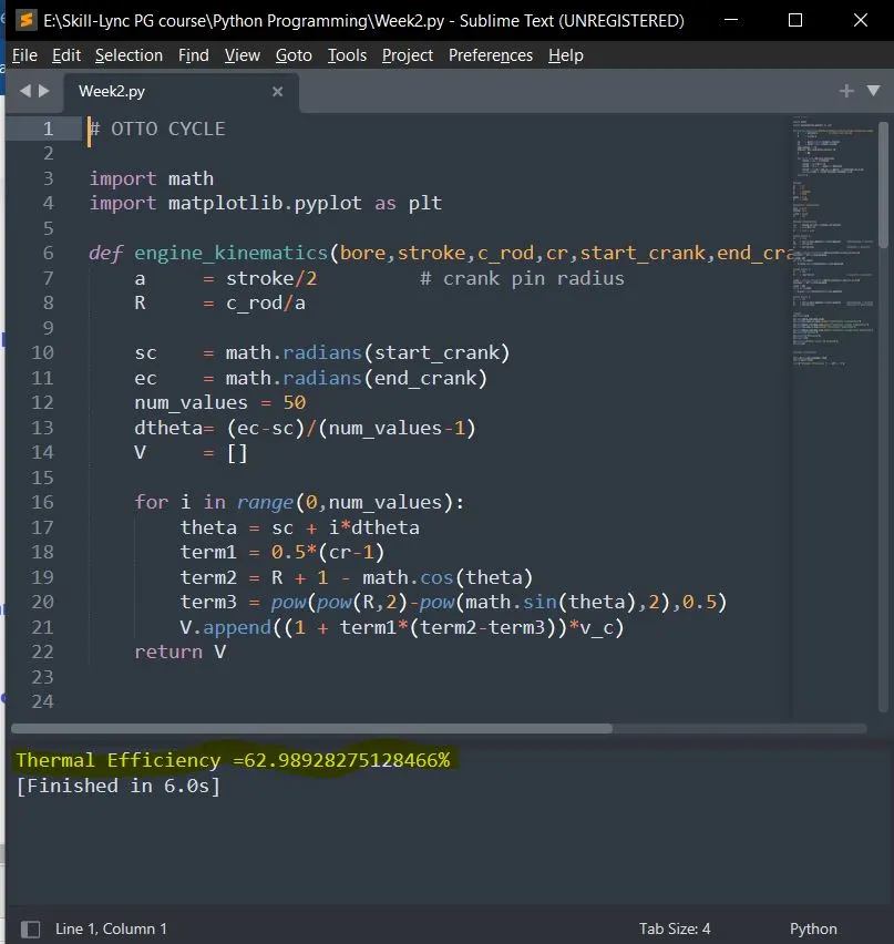
Inference : The value of Thermal Efficiency which was calculated in the program is displayed in the output window (Highlighted )