Week 2 Air standard Cycle

Based on the concepts you have learnt during the forward kinematics routine, go ahead and write code that can solve an otto cycle and make plots for it.

Here are the requirements

1. Your code should create a PV diagram

2. You should output the thermal efficiency of the engine.

The four processes in an Otto cycle are:

1. Isentropic compression process or Reversible adiabatic compression of air (Process 1-2),
2. Constant volume heat addition process (Process 2-3),
3. Isentropic expansion process or Reversible adiabatic expansion of air (Process 3-4),
4. Constant volume heat rejection process (Process 4-1).

GOVERNING EQUATIONS :

Various equations of Otto cycle are involved in this project. These are :

• Compression ratio (rc">rcrc) , rc=(V1V2)">rc=(V1V2)rc=(V1V2) or 1+VsVc">1+VsVc1+VsVc,

• Swept volume (Vs">VsVs) = π4⋅d2⋅l">π4⋅d2⋅lπ4⋅d2⋅l, where d is bore diameter and l is stroke length,

• VVc">VVcVVc = 1 + 12(rc-1)[R+1-cosθ-(R2-sin2θ)12]">12(rc−1)[R+1−cosθ−(R2−sin2θ)12]12(rc-1)[R+1-cosθ-(R2-sin2θ)12],

where R = length of connecting rod/crank radius ,

• Adiabatic process equation = p⋅vγ">p⋅vγp⋅vγ = constant,

• Ideal Gas equation = p⋅v=m⋅R⋅T">p⋅v=m⋅R⋅Tp⋅v=m⋅R⋅T,

• Thermal efficiency of Otto cycle(η">ηη)= 1-1rcγ-1">1−1rγ−1c1-1rcγ-1,

• From the figure, v1">v1v1 = vs+vc">vs+vcvs+vc , v2=vc">v2=vcv2=vc.

PYTHON CODE

# Otto Cycle Simulator

import math
import matplotlib.pyplot as plt

def engine_kinematics(bore,stroke,con_rod,cr,start_angle,end_angle):
	# Engine Parameters
	a = stroke/2
	R = con_rod/a

	# Volume Computation
	v_s = (math.pi/4)*pow(bore,2)*stroke
	v_c = v_s/(cr-1)

	sc = math.radians(start_angle)
	ec = math.radians(end_angle)

	num_values = 50
	dtheta = (sc-ec)/(num_values-1)
	v = []
	for i in range(0,num_values):
		theta = sc+i*dtheta
		term1 = 0.5*(cr-1)
		term2 = R+1-math.cos(theta)
		term3 = pow(R,2)- pow(math.sin(theta),2)
		term3 = pow(term3,0.5)
		v.append((1+term1*(term2-term3))*v_c)

	return v

# Inputs
p1 = 101325
t1 = 500
gamma = 1.4
t3 = 2300

# engine parameters
bore = 0.1
stroke = 0.1
con_rod = 0.15
cr = 8

# Volume Computation
v_s = (math.pi/4)*pow(bore,2)*stroke
v_c = v_s/(cr-1)
v1 = v_s + v_c

# Stage2
v2 = v_c

p2 = p1*pow(v1,gamma)/pow(v2,gamma)
rhs = p1*v1/t1
t2 = p2*v2/rhs
v_compression = engine_kinematics(bore,stroke,con_rod,cr, 180, 0)

constant = p1*pow(v1,gamma)

p_compression = []

for v in v_compression:
	p_compression.append(constant/pow(v,gamma))

# Stage3
v3 = v2
rhs = p2*v2/t2
p3 = rhs*t3/v3

v_expansion = engine_kinematics(bore,stroke,con_rod,cr,0,180)

constant = p3*pow(v3,gamma)

p_expansion = []

for v in v_expansion:
	p_expansion.append(constant/pow(v,gamma))

# Stage4
v4 = v1

p4 = p3*pow(v3,gamma)/pow(v4,gamma)

t4 = p4*v4/rhs

# Thermal efficiency
n = 1 - (pow(cr,(1-gamma)))
print(n)

plt.plot([v2,v3],[p2,p3])
plt.plot(v_compression,p_compression)
plt.plot(v_expansion,p_expansion)
plt.plot([v4,v1],[p4,p1])
plt.xlabel('Volume')
plt.ylabel('Pressure')
plt.show()

BODY OF THE CONTENT :

EXPLANATION OF PYTHON CODES :

1. Since the Otto cycle is an air-standard cycle, the specific heat of air is taken as 1.4.
2. Initial conditions, such as temperature (T1">T1T1)and pressure (p1">p1p1) of the surrounding is assumed to be 350K and 101.325 kPa respectively.
3. The geometrical design of the engine cylinder which consists of bore diameter, stroke length, and length of connecting rod is also known and accordingly vs">vsvs and vc">vcvc are calculated.
4. The maximum temperature (T3">T3T3) occurring inside the cylinder is also known.
5. Other state variables are calculated using Adiabatic processes equations and ideal gas equations.
6. Similarly, the thermal efficiency is also calculated accordingly using the formula given.
7. For plotting the calculated state variables on a p-v diagram with just using 'plt.plot' the command will yield into the incorrect p-v diagram,i.e, compression and expansion stroke is represented by a straight line.
8. So to rectify this, a different function is created for storing the different values of crank angle rotation as compression and expansion occur in different strokes or cycles. This function is then called to the main program and accordingly, the plot is drawn from various points obtained.
9. For this number of values for which the program will iterate is 100, and accordingly, the V array is set as null and after every iteration using for loop, a new value will be stored as an array using 'append' command and will be returned back after receiving desired values.

RESULTS :

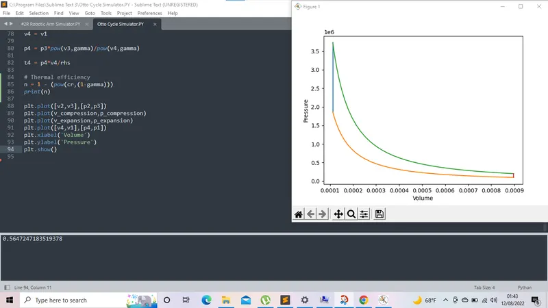
the following plot for the p-V curve

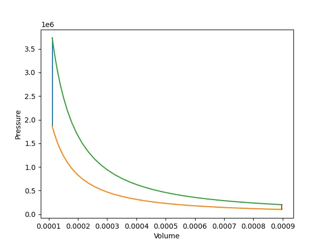
Thermal efficiency of the engine = 56.47 %

Main Window